`geom_smooth()` using formula = 'y ~ x'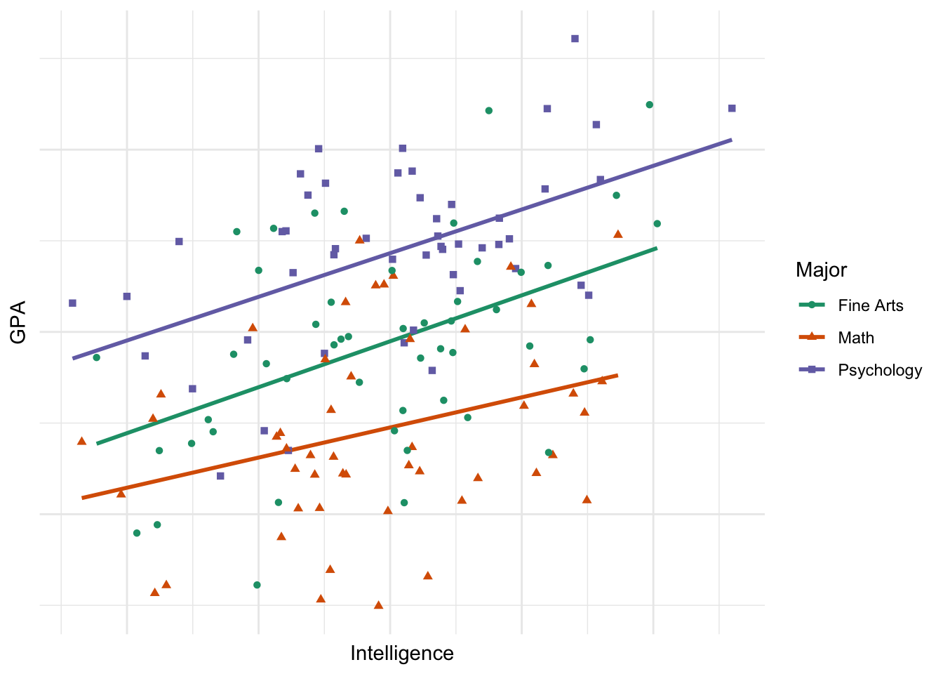
Analysis of Covariance (ANCOVA) focuses on accounting for variance explained by a continuous variable that may not be the maniupulated or pseudo-manipulate variable of interest. Thus, we expend our ANOVA to account for another variable. Typically, we call this other variable a covariate.
Simply, we include a covariate in model predicting the DV, without the IV. Then, we add the IV to determine if it has an effect above and beyond the covariate. Furthermore, adding a covariate can help reduce the error variance (i.e., it explains what would otherwise be unexplained error variance). Last, adding a covariate can reduce the impact of confounds on the DV by including them as covariates.
An ANCOVA is essentially a model with a continuous covariate and a dummy coded IV.
\(y_i=(model)+e_i\)
\(y_i=b_0+b_{1}(x_{1i})+b_2({x_{2i}})+e_i\)
Where \(b_1\) is the regression coefficient for the covariate, \(x_{1i}\) is individual \(i\)’s score on the covariate, \(b_2\) is the coefficient for the dummy coded IV, \(x_{2i}\) is individual \(i\)’s score on the IV (0 or 1), and \(e_i\) is the error.
Note that there will be more dummy coefficients for more levels of the IV (number of dummy coded variables = levels - 1). For example, if we were conducting a study with one covariate and an IV with three levels (low, medium, and high), our resulting model would be:
\(y_i = b_0+b_1(x_{covariate})+b_2(x_{medium})+b_3(x_{high})\)
ANCOVA has two assumptions that we have not encountered.
If the ANOVA model, covariate ~ IV is statistically significant, it would indicate the the covariate differs between IV levels to a degree that is unlikely under a true null hypothesis of equal covariates between levels of the IVs. Thus, the covaiate and the I are not independent.
We want a non-statsitically significant result for this test.
`geom_smooth()` using formula = 'y ~ x'
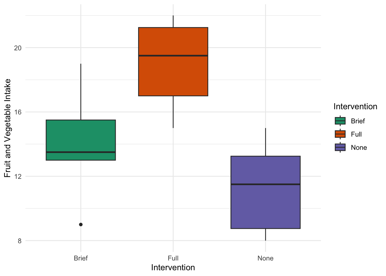
You are hired by an organization seeking to promote healthy families in the community. They are implementing a course for families around healthy nutrition and balanced diets. They are interested in the impact of participating in a full version of this course, a brief version, and no treatment (three-level IV) on eating habits (DV). Specifically, will measure eating habits as the total number of servings of fruits/vegetables per family over a one week period, divided by the number of people in that family. Thus, a DV score of 12 would indicate that the family ate total 12 servings of fruits or vegetables per person over the week following their intervention. They ask you to conduct the analyses. Importantly, you know that income is a strong predictor of eating habits, because healthy foods are typically more expensive. Thus, you treat income as a covariate (family income/year).
What are the IV, DV, and covariate?
What could be another covariate?
What is the model (i.e., write out the regression equation)?
IV: eating intervention. Three levels (full, brief, none). DV: average fruit and vegetables intake per person in a family over one week. Covariate: income.
Many possibilities.
\(y_{fruitvegetable,i}=b_0+b_i(x_{income,i})+b_2(x_{full,i})+b_3(x_{brief,i})+e_i\)
You review the literature and determine find a nice meta-analysis on eating habit interventions. This study suggests that a brief intervention was able to effectively reduce junk food consumption and resulted in a effect size if \(\eta^2=.54\), \(95\%CI[.35, .62]\). Bring brilliant, you use the lower bound estimate. Your power analysis suggests:
pwr.anova.test(k = 3,
         f = sqrt((.35)/(1-.35)), ## remember, f2 = square root of eta2/(1-eta2)
         power = .8)
     Balanced one-way analysis of variance power calculation

              k = 3
              n = 7.065318
              f = 0.7337994
      sig.level = 0.05
          power = 0.8

NOTE: n is number in each group
Thus, we need eight families per group. You successfully recruit 24 families. You obtain the following data:
| Family | Intervention | FV | Income |
|---|---|---|---|
| 1 | Full | 18 | 57200 |
| 2 | Full | 15 | 57900 |
| 3 | Full | 21 | 62100 |
| 4 | Full | 21 | 55200 |
| 5 | Full | 22 | 50700 |
| 6 | Full | 17 | 62900 |
| 7 | Full | 17 | 60500 |
| 8 | Full | 22 | 51500 |
| 9 | Brief | 14 | 50500 |
| 10 | Brief | 13 | 59500 |
| 11 | Brief | 13 | 44200 |
| 12 | Brief | 17 | 61900 |
| 13 | Brief | 13 | 47400 |
| 14 | Brief | 9 | 55500 |
| 15 | Brief | 19 | 50500 |
| 16 | Brief | 15 | 57800 |
| 17 | None | 9 | 52100 |
| 18 | None | 8 | 48100 |
| 19 | None | 12 | 57200 |
| 20 | None | 11 | 46000 |
| 21 | None | 13 | 65300 |
| 22 | None | 8 | 49400 |
| 23 | None | 15 | 50400 |
| 24 | None | 14 | 50000 |
Which would result in the following descriptives:
Descriptive statistics for FV as a function of Intervention.

 Intervention     M   SD
        Brief 14.12 3.00
         Full 19.12 2.70
         None 11.25 2.71

Note. M and SD represent mean and standard deviation, respectively.
Our hypothesis will be analogous to one-way ANOVA.
\(H_O: \mu_{none}=\mu_{brief}=\mu_{full}\) (or, all \(\mu\)s equal)
\(H_A=\) at least one \(\mu\) different
First, let’s check our assumptions.
mod_independence <- aov(Income ~ Intervention, data=dat_nutr)

apa.aov.table(mod_independence, conf.level = .95)
ANOVA results using Income as the dependent variable


    Predictor             SS df             MS      F    p partial_eta2
  (Intercept) 22823161250.00  1 22823161250.00 699.71 .000
 Intervention   107507500.00  2    53753750.00   1.65 .216          .14
        Error   684977500.00 21    32617976.19
 CI_95_partial_eta2

         [.00, .36]


Note: Values in square brackets indicate the bounds of the 95% confidence interval for partial eta-squared
Thus, we have not violated the assumptions. The income level did not differ based on treatment groups, \(F(2, 21) = 1.65\), \(p = 0.216\); \(\eta^2 = 0.14\), \(95\%CI[0.00, 0.31]\).
We want to test a model including both covariate, DV, and their interaction. We will interpret our main analyses later, but for now, focus on the interaction term in a full ANOVA model. We will specify an interaction by simply multiplying the DV and covariate in a model (in addition to our regular model). We must specify a type 3 sums of squares. We will the the apa.aov.table() function from the apaTables package:
homogeneity_regression_slope_model <- aov(FV ~ Intervention + Income + Intervention*Income, data=dat_nutr)

apa.aov.table(homogeneity_regression_slope_model, type=3, conf.level = .95)
ANOVA results using FV as the dependent variable


             Predictor     SS df    MS    F    p partial_eta2
           (Intercept)  12.11  1 12.11 1.55 .230
          Intervention  39.10  2 19.55 2.50 .110          .22
                Income   0.72  1  0.72 0.09 .765          .01
 Intervention x Income  24.34  2 12.17 1.55 .238          .15
                 Error 140.91 18  7.83
 CI_95_partial_eta2

         [.00, .45]
         [.00, .19]
         [.00, .38]


Note: Values in square brackets indicate the bounds of the 95% confidence interval for partial eta-squared
We want to focus on the interaction term. Here the interaction (Intervention x Income) is not statistically significant. This indicates that the relationship between income and FV consumed does not depend on intervention type. We have not violated the assumption.
In my opinion, it makes much more sense to do this after your main ANCOVA analysis because you are, essentially, running an ANCOVA here with an extra interaction term.
leveneTest(lm(FV~Intervention, data=dat_nutr))Levene's Test for Homogeneity of Variance (center = median)
Df F value Pr(>F)
group 2 0.0544 0.9472
21 We conducted Levene’s test to asses the homogeneity of variances and the results suggest that we did not violate this assumption, \(F(2, 21)=.054\), \(p=.9472\).
ezANOVA()We will not calculate ANOCOVA by hand. Instead, we will use R. We can use a number of functions to calculate the ANCOVA; however, the ezANOVA() function from the ez package is, not to sound lame, ez. We will need to specify the type of sum of squares; we will use type 2 because we don’t care about an interaction. Note that this function will run Levene’s test on the adjusted data.
library(ez)
ezANOVA(data=dat_nutr,
        between = Intervention,
        dv = FV,
        between_covariates = Income,
        wid=Family,
        type=2,
        detailed = T)
$ANOVA
Effect DFn DFd SSn SSd F p p<.05 ges
1 Intervention 2 21 191.2115 194.3071 10.33272 0.0007510256 * 0.4959852
$`Levene's Test for Homogeneity of Variance`
DFn DFd SSn SSd F p p<.05
1 2 21 3.997507 68.09335 0.6164159 0.5493604 aov()We could use the default aov() to conduct our analyses. The lovely apa.aov.table() function let’s us specify the types of sums of squares. We will use the apa.aov.table() output for our class.
our_full_model <- aov(FV ~ Income + Intervention, data=dat_nutr)

apa.aov.table(our_full_model, type = 2)
ANOVA results using FV as the dependent variable


    Predictor     SS df     MS     F    p partial_eta2 CI_90_partial_eta2
       Income   0.00  1   0.00  0.00 .996          .00
 Intervention 220.27  2 110.14 13.33 .000          .57         [.26, .69]
        Error 165.25 20   8.26

Note: Values in square brackets indicate the bounds of the 90% confidence interval for partial eta-squared
Thus, it seems the covariate, income, is not linked to the amount of FV consumed. However, there is a main effect of intervention on number of F&V consumed.
Although the apa.aov.table() function can calculate our effect size for us, we should know what it means. We can calculate \(\eta^2_p\) (partial eta squared). \(\eta^2_p\) can be calculated as:
\(\eta^2_p = \frac{SS_{effect}}{SS_{effect}+SS_{error/residual}}\)
For our intervention:
\(\eta^2_p=\frac{220.27}{220.27+165.25}=.571\)
This represent a ratio of what is explained by the IV compared to the residual error.
Much like a one-way ANOVA, we will need to conduct post-hoc tests. However, we will need to adjust the groups to account for any differences in covariates; remember, we want to control for these differences in the DV, which is why we are doing this in th first place. We can still use Tukey’s HSD, but we will need to use a different function. Specifically, we will use the glht() function from the multcomp package. This will return the post-hoc Tukey comparison of each group.
library(multcomp)

post_hoc <- glht(our_full_model, linfct = mcp(Intervention = "Tukey"))

summary(post_hoc)
     Simultaneous Tests for General Linear Hypotheses

Multiple Comparisons of Means: Tukey Contrasts


Fit: aov(formula = FV ~ Income + Intervention, data = dat_nutr)

Linear Hypotheses:
                  Estimate Std. Error t value Pr(>|t|)
Full - Brief == 0    4.998      1.498   3.337  0.00876 **
None - Brief == 0   -2.874      1.442  -1.993  0.13971
None - Full == 0    -7.872      1.536  -5.125  < 0.001 ***
---
Signif. codes:  0 '***' 0.001 '**' 0.01 '*' 0.05 '.' 0.1 ' ' 1
(Adjusted p values reported -- single-step method)
And the associated confidence intervals using the following:
confint(post_hoc)
     Simultaneous Confidence Intervals

Multiple Comparisons of Means: Tukey Contrasts


Fit: aov(formula = FV ~ Income + Intervention, data = dat_nutr)

Quantile = 2.5277
95% family-wise confidence level


Linear Hypotheses:
                  Estimate lwr      upr
Full - Brief == 0   4.9977   1.2118   8.7836
None - Brief == 0  -2.8743  -6.5201   0.7714
None - Full == 0   -7.8720 -11.7550  -3.9891
It is also important to get effect size estimates for each comparison. But remember, we want to adjust the means using the covariate (i.e., account for their different scores on the covariate). We can do this using the mes() function from the copmute.es package. We will also need the adjusted means and standard deviations.
library(effects)

## Get the adjusted means for our model
adjusted <- effect("Intervention", our_full_model, se=T)

## Means
summary(adjusted)
 Intervention effect
Intervention
   Brief     Full     None
14.12555 19.12324 11.25121

 Lower 95 Percent Confidence Limits
Intervention
    Brief      Full      None
11.995358 16.899938  9.081744

 Upper 95 Percent Confidence Limits
Intervention
   Brief     Full     None
16.25574 21.34654 13.42068
We will also need adjusted standard deviations. We have standard errors:
## Standard errors (will be used later)
adjusted$se
[1] 1.021203 1.065839 1.040032Note: the order aligns with the previous adjusted means (Brief, Full, None). You may recall from an earlier chapter that \(\sigma_{\overline{x}=\frac{s}{\sqrt{N}}}\). Thus, we can estimate:
\(s=\sigma_\overline{x}\sqrt{N}\)
We have eight per group, thus the following will return the adjusted SD for each group:
adjusted$se*sqrt(8)[1] 2.888397 3.014648 2.941653Again, the order aligns with the output from the adjusted means (Brief, Full, None). The mes() function can then calculate each standardized difference (Cohen’s d) for each group difference.
library(compute.es)

## Brief vs Full
mes(m.1 = 14.12555,
    m.2 = 19.12324,
    sd.1 = 2.888397,
    sd.2 = 3.014648,
    n.1 = 8,
    n.2 = 8)
Mean Differences ES:
d [ 95 %CI] = -1.69 [ -2.83 , -0.55 ]
var(d) = 0.34
p-value(d) = 0.01
U3(d) = 4.52 %
CLES(d) = 11.56 %
Cliff's Delta = -0.77
g [ 95 %CI] = -1.6 [ -2.68 , -0.52 ]
var(g) = 0.3
p-value(g) = 0.01
U3(g) = 5.47 %
CLES(g) = 12.89 %
Correlation ES:
r [ 95 %CI] = -0.67 [ -0.88 , -0.26 ]
var(r) = 0.02
p-value(r) = 0.01
z [ 95 %CI] = -0.81 [ -1.36 , -0.27 ]
var(z) = 0.08
p-value(z) = 0.01
Odds Ratio ES:
OR [ 95 %CI] = 0.05 [ 0.01 , 0.37 ]
p-value(OR) = 0.01
Log OR [ 95 %CI] = -3.07 [ -5.14 , -1 ]
var(lOR) = 1.12
p-value(Log OR) = 0.01
Other:
NNT = -5.14
Total N = 16## Brief vs None
mes(m.1 = 14.12555,
m.2 = 11.25121,
sd.1 = 2.888397,
sd.2 = 2.941653,
n.1 = 8,
n.2 = 8)Mean Differences ES:
d [ 95 %CI] = 0.99 [ -0.05 , 2.02 ]
var(d) = 0.28
p-value(d) = 0.08
U3(d) = 83.79 %
CLES(d) = 75.72 %
Cliff's Delta = 0.51
g [ 95 %CI] = 0.93 [ -0.05 , 1.91 ]
var(g) = 0.25
p-value(g) = 0.08
U3(g) = 82.44 %
CLES(g) = 74.51 %
Correlation ES:
r [ 95 %CI] = 0.47 [ -0.04 , 0.78 ]
var(r) = 0.04
p-value(r) = 0.09
z [ 95 %CI] = 0.51 [ -0.04 , 1.05 ]
var(z) = 0.08
p-value(z) = 0.09
Odds Ratio ES:
OR [ 95 %CI] = 5.98 [ 0.91 , 39.28 ]
p-value(OR) = 0.08
Log OR [ 95 %CI] = 1.79 [ -0.09 , 3.67 ]
var(lOR) = 0.92
p-value(Log OR) = 0.08
Other:
NNT = 2.8
Total N = 16#Full vs None
mes(m.1 = 19.12324,
m.2 = 11.25121,
sd.1 = 3.014648,
sd.2 = 2.941653,
n.1 = 8,
n.2 = 8)Mean Differences ES:
d [ 95 %CI] = 2.64 [ 1.3 , 3.98 ]
var(d) = 0.47
p-value(d) = 0
U3(d) = 99.59 %
CLES(d) = 96.92 %
Cliff's Delta = 0.94
g [ 95 %CI] = 2.5 [ 1.23 , 3.77 ]
var(g) = 0.42
p-value(g) = 0
U3(g) = 99.38 %
CLES(g) = 96.14 %
Correlation ES:
r [ 95 %CI] = 0.82 [ 0.54 , 0.93 ]
var(r) = 0.01
p-value(r) = 0
z [ 95 %CI] = 1.15 [ 0.6 , 1.69 ]
var(z) = 0.08
p-value(z) = 0
Odds Ratio ES:
OR [ 95 %CI] = 120.78 [ 10.6 , 1375.76 ]
p-value(OR) = 0
Log OR [ 95 %CI] = 4.79 [ 2.36 , 7.23 ]
var(lOR) = 1.54
p-value(Log OR) = 0
Other:
NNT = 1.31
Total N = 16We investigated the impact of a healthy eating intervention on the average number of fruits and vegetables consumed per person, per family over the course of one week. Additionally, we controlled for family income. We hypothesized that intervention would impact the amount of F&V consumed and explored potential differences using post-hoc comparisons. We tested several assumptions to determine the suitability of ANCOVA to test our hypothesis.
The assumption of independence of intervention and our covariate, income was held. The income level did not differ based on treatment groups, \(F(2, 21) = 1.65\), \(p = 0.216\); \(\eta^2 = 0.14\), \(95\%CI[0.00, 0.31]\). Second, we conducted Levene’s test to assess the homogeneity of variances of treatment groups; the results suggest that we did not violate this assumption, \(F(2, 21)=.054\), \(p=.9472\). Last, we did not violate the homogeneity of regression slope assumption, \(F(2, 18)=1.55\), \(p=.238\).
We conducted an ANCOVA to determine the impact of intervention on consumption of fruits and vegetables, using family income as a covariate. The covariate, income, was not related to the consumption of fruits or vegetables, \(F(1, 20)= 0.00\), \(p=.996\), \(\eta^2_p= 0\). However, the results suggest the amount of fruit and vegetables consumed did vary by treatment type to a proportion that is unlikely given a true null hypothesis \(F(2, 20)= 110.14\), \(p<.001\), \(\eta^2_p= .57\), \(95\%CI[.26, .69]\).
We conducted post-hoc tests using Tukey’s LSD to determine which interventions differed. We had no a priori hypothesis; thus, we analyses were purely exploratory. First, our results suggest that families in the Full intervention (\(M=19.12\)) consumed statistically significant more fruits and vegetables compared to the Brief intervention (\(M=14.13\)), difference \(= 4.99\), \(d=1.69\), \(95\%CI=[0.55, 2.83]\), \(p=.001\).
Second, our results suggest that families in the Full intervention (\(M=19.12\)) consumed statistically significant more fruits and vegetables compared to no intervention (\(M=11.25121\)), difference \(= 7.87\), \(d=2.64\), \(95\%CI=[1.30, 3.98]\), \(p<.001\).
Third, our results suggest that families in the Full intervention (\(M=11.25121\)) consumed statistically significant more fruits and vegetables compared to the Brief intervention (\(M=14.13\)), difference \(= 2.87\), \(d=0.99\), \(95\%CI=[-0.05, 2.02]\), \(p=.139\).