You are hired by Instagram to research their trending posts. They ask if people like more posts based on the poster’s attractiveness. You decide that you will collect posts and determine if there is a relationship between the number of likes a posts receives and how attractive the poster is rated.
16.1.1 Power Analysis
You review the literature and determine that the there is a strong link between attractiveness and popularity. You determine the best estimate to of a population parameter to be \(\rho=.75\). You power analysis (see chapter related to power) results in:
pwr.r.test(r = .75,power = .8,sig.level = .05)
     approximate correlation power calculation (arctangh transformation)

              n = 10.72495
              r = 0.75
      sig.level = 0.05
          power = 0.8
    alternative = two.sided
Thus, you collect 11 posts largely featuring one person. You average the attractiveness ratings of 4 independent raters and get the following data.
Likes
Attractiveness
22272
8
47387
10
65
3
417
4
99
3
143
5
41123
8
108
5
28183
3
330
1
21268
7
16.2 Our Hypothesis
We hypothesize that there is a relationship between attractiveness and likes of a post. Thus, our hypotheses are as follows under NHST. Note: \(\rho\) (‘row’) is the population correlation.
\(H_0:\rho=0\)
\(H_A:\rho\neq0\)
16.3 Our Analysis
16.3.1 Covariance
We typically estimate the associations with variables using covariances and correlations. Prior to looking at correlations, let’s discuss covariance. The coravariance measures the cross-product (multiplication of two variables) or deviations to determine the average deviations. Consider the mean for likes 1.4672273^{4} and attractiveness 5.1818182. We would calculate how much each variables deviates from the mean, mulitple each, then average them.
A positive covariance indicates that the variables tend to associate in the same direction. So here, posts with more likes tend to be rated as more attractiveness. A negative covariance would indicate the opposite: higher scores on one variable are associated with lower scores on others.
A major issue with covariance is that it is not standardized. That is, it is difficult to compare covariances with one another. This makes them difficult to interpret. One cannot readily interpret a covariance of 10, 100, 1000, or 10000, because they depend on the metric of the variables used to calculate it. For example, imagine that I wanted to calculate the covariance of height and weight (kg). I could use cm or m as a metric of height. When I use height in cm I get a covariance of 189.44. When I use height in m, I get 1.89. This is despite the strength of the association being identical. How might we resolve this?
16.3.2 Correlation Coefficient
The correlation coefficient is a standardized covariance. What does standardization do? It converts a variable into a standard unit that facilitates comparisons. We can scale our variables considering the standard deviations. Specifically, we would adjust our formula to be:
\(r=\frac{cov_{x,y}}{s_xs_y}\)
Which, can be re-written as:
\(r=\frac{SP}{\sqrt{(SS_x)(SS_y)}}\)
Where \(SS_x\) is the sum of squared deviations of x and \(SS_y\) is the sum of squared deviations of y.
Thus, using our data above, we need the standard deviation of Likes (18197.74) and Attractiveness (2.75). Thus, using covariance and standard deviations:
\(r=\frac{38188.05}{(18197.74)(2.75)}=.763\)
Or, if we used sum of squared deviations (the second way to calculate it; see above):
Correlation have some important properties. First, they range from -1 to 1. A correlation of -1 indicates a perfect negative relationship. A correlation of 1 indicates a perfect positive relationship. A correlation of 0 indicates no relationship. Thus, correlation helps us understand the direction (+, -) and magnitude (absolute size of the number) of a relationship. For example, \(r=.4\) indicates a positive relationship, but \(r=-.6\) indicates a stronger negative relationship.
For our research, seems that Likes and Attractiveness have a strong positive relationship. However, you know that we must determine if this data is unlikely given a true null hypothesis.
16.3.3 Distirbution of r
Correlations have a distribution that is related to the t distribution. Simply, r can be converted to a t value:
\(t_r=\frac{r\sqrt{(n-2)}}{\sqrt{1-r^2}}\)
We could then use a t-distribution to determine the likelihood of our or more extreme data given a true null. For our example:
Looking up the in our t-distribution table, we get a p-value of .00629. Therefore, our probability of getting this large or larger of a correlation under a true null is 0.006.
16.4 Our r in R
We can use the cor.test() function, where we specify the two variables we wish to correlate.
cor.test(dat$Likes, dat$Attractiveness) #our data was called 'dat'
    Pearson's product-moment correlation

data:  dat$Likes and dat$Attractiveness
t = 3.5416, df = 9, p-value = 0.006299
alternative hypothesis: true correlation is not equal to 0
95 percent confidence interval:
 0.3008816 0.9349566
sample estimates:
      cor
0.7630353
Note that R provides many useful pieces of information: \(r\), \(t\), and \(p\). It also gives us the 95%CI (which is for \(r\)). You can use r as an effect size, but \(R^2\) (squaring \(r\)), the coefficient of determination, also indicates the proportion in one variable that is explained by the other. Here, 58.22% of the variance in Likes can be explained by knowing the Attractiveness rating of the poster. Note: this doesn’t mean causes. It means by knowing someones Attractiveness/Likes, we have a fairly reliable guess at what the other would be.
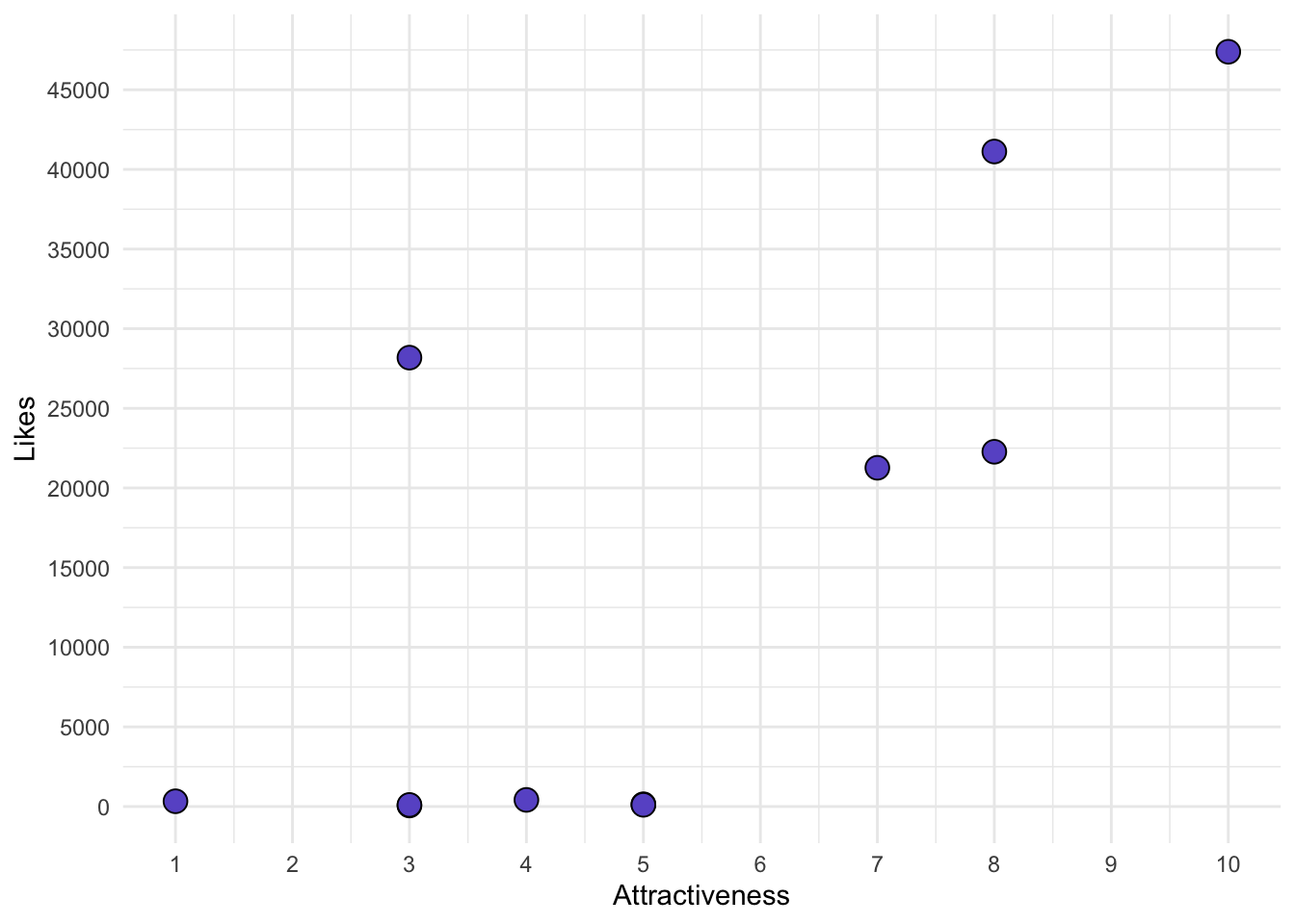
16.5 Plotting
The standard way to plot two continuous variables is through a scatterplot.
It’s important to visually inspect your data. The datasauRus package shows a quick demonstration how data can look vastly different with the exact same means, standard deviations, and correlations. As is the case for each of the following datasets:
16.6 Our Results
We hypothesized that the number of likes on an Instagram post would be correlated with the rated Attractiveness of the poster. The results suggest that our data are unlikely given a true null hypothesis, \(r=.763\), \(95\%CI[.30, .93]\), \(df=9\), \(p=.006\), \(R^2=.582\). Approximately 58.2% of the variance in Likes can be explained by Attractiveness, indicating a strong effect size.
16.7 Our Assumptions
The data are continuous.
There are other types of correlation, but they will not be discussed here. Future updates may include them.
16.8 Practice Questions
Practice Questions
Using the following data, which were measurements of sizes of children’s books:
Height
Width
10
4
9
11
18
16
4
6
15
20
12
13
11
16
9
12
Calculate the correlation, and write the results up (including \(r\), \(p\), and the CI if you use R).
Draw a quick scatterplot of the data (put width on the x-axis).
Answers
Warning: package 'report' was built under R version 4.3.3
Warning: Function `format_text()` is deprecated and will be removed in a future
  release. Please use `text_format()` instead.
Effect sizes were labelled following Funder's (2019) recommendations.

The Pearson's product-moment correlation between df_prac$Height and
df_prac$Width is positive, statistically significant, and very large (r = 0.72,
95% CI [0.04, 0.95], t(6) = 2.56, p = 0.043)