22  Non-parametrics

In progress. Check back soon.

22.1 Parametric versus Nonparametric Statistics

Parametric statistical methods involve making assumptions about the distribution of the population or its parameters. These assumptions are typically explicit, such as assuming data follows a normal distribution, exhibits homogeneity of variance, and that observations are independent. We have covered many of these assumptions through other parametric tests within the general linear model. Parametric methods dominate much of the psychological literature, where researchers often rely on these assumptions to draw conclusions about the data. By assuming a specific form for the underlying population distribution, parametric methods can provide precise estimates of parameters and perform hypothesis tests with greater statistical power. However, the validity of parametric methods relies heavily on the accuracy of these assumptions, which may not always hold true in real-world scenarios.

Non-parametric statistical methods operate under the premise of being distribution-free or making minimal assumptions about the underlying population distribution. Unlike parametric methods, non-parametric techniques do not rely on specific distributional assumptions such as normality, homogeneity of variance, or independence of observations. Instead, they are designed to be more flexible and applicable in situations where these assumptions may not hold true. While non-parametric methods are less common compared to parametric approaches, they have important applications, particularly in cases where the data distribution is unknown or cannot be assumed to follow a particular pattern. These methods offer valuable tools for analyzing data in a wide range of fields, providing robustness and reliability in scenarios where traditional parametric techniques may be inadequate.

22.2 Traditional Non-parametrics

In traditional non-parametric methods, a key approach involves ranking the data. This technique is employed to remove the influence of extreme values and to work with the ordinal nature of the data rather than its exact values. Ranking data offers predictable properties, such as the sum of ranks of a dataset being equal to \(N\times \frac{(N+1)}{2}\), where \(N\) represents the total number of observations. This property aids in simplifying calculations and understanding the distribution of ranks within the dataset. Moreover, critical values derived from ranked data tend to be less convoluted compared to those from raw data, making them easier to interpret and apply in statistical analyses.

Consider an example with two groups, each consisting of three people, making \(N=6\) individuals in total. Consider the following possible ranks for one group of three individuals:

Scenario	Person1	Person2	Person3	Sum
1	1	2	3	6
2	1	2	4	7
3	1	2	5	8
4	1	2	6	9
5	1	3	4	8
6	1	3	5	9
7	1	3	6	10
8	1	4	5	10
9	1	4	6	11
10	1	5	6	12
11	2	3	4	9
12	2	3	5	10
13	2	3	6	11
14	2	4	5	11
15	2	4	6	12
16	2	5	6	13
17	3	4	5	12
18	3	4	6	13
19	3	5	6	14
20	4	5	6	15

Another, perhaps more simple way to conceptualize the potential sum of ranks of these individuals can be calculated. When considering one group with \(n=3\) individuals, the possible sums of ranks range from \(1 + 2 + 3 = 6\) (if all individuals are ranked consecutively at the top of the ranks) to \(4 + 5 + 6 = 15\) (if all individuals are ranked consecutively at the bottom of the ranks). Thus, the possible sum of ranks for one group, where \(n=3\), ranges from 6 to 15 inclusive.

To help determine the probability of obtaining a specific sum of ranks, let’s we can calculate cumulative frequencies.

Sum	Count	Cumulative_Frequency	Cumulative_Percentage
6	1	1	5
7	1	2	10
8	2	4	20
9	3	7	35
10	3	10	50
11	3	13	65
12	3	16	80
13	2	18	90
14	1	19	95
15	1	20	100

As can be seen, only 5% of the time would we expect (if rankings were random) to obtain rankings 1, 2, and 3 (a sum of 6) for our three-person group. Using this knowledge, we can complete hypothesis testing under a ‘null’, much as we did for our general linear models (e.g., t-tests, ANOVAs, regressions).

22.2.1 Wilcoxon-Mann-Whitney Rank Sum Test

The Wilcoxon-Mann-Whitney Rank Sum Test, often referred to simply as the Rank-Sum Test, serves as a non-parametric alternative to the t-test for comparing differences between two independent groups. This test operates by either using the ranks of the data directly or by replacing the actual data with ranks. In cases where ties occur, the ranks should be adjusted to account for these instances, typically by assigning tied values the average of the ranks they would have received. For instance, if two individuals both have a rank of 4 (which would be, in order, counted as rank 4 and 5), their ranks are adjusted to 4.5 each (\(\frac{4+5}{2}=4.5\). This adjustment ensures fairness and accuracy in the ranking process.

The Rank-Sum Test is particularly useful when data violate assumptions such as homogeneity of variance, when dealing with very small sample sizes, or when working with ordinal data where the assumptions of parametric tests are not met. By relying on the ranks of the data rather than their exact values, this test provides a robust method for comparing groups without requiring stringent distributional assumptions.

22.2.1.1 An Example - Drug Efficacy

Imagine we have developed a drug to enhance cognitive function. Specifically, we randomly assign participants to either the drug or control group. Subsequently, their cognitive performance is measured using a standardized test. After performing some diagnostic checks on the data, we conclude that the distribution of cognitive performance seems to have violated the homogeneity of variance assumptions. Instead of relying on the traditional parametric tests, an independent samples t-tests, the Rank-Sum Test offers a robust alternative. By comparing the ranks of cognitive test scores between the drug and control groups, this non-parametric test effectively assesses whether the drug has a significant impact on cognitive function.

Here is our data:

ID	Group	Score
1	Control	14.74
2	Control	19.04
3	Control	11.56
4	Control	10.19
5	Control	13.68
6	Experimental	19.13
7	Experimental	14.44
8	Experimental	19.32
9	Experimental	24.97
10	Experimental	21.78

22.2.2 Rank-Sum Test

In the context of the Rank-Sum Test, if the ranks assigned to individuals are essentially “random,” the sum of ranks should be approximately equal for each group under comparison. As an initial step, let’s rank our data:

ID	Group	Score	Rank
1	Control	14.74	6
2	Control	19.04	5
3	Control	11.56	9
4	Control	10.19	10
5	Control	13.68	8
6	Experimental	19.13	4
7	Experimental	14.44	7
8	Experimental	19.32	3
9	Experimental	24.97	1
10	Experimental	21.78	2

The Rank-Sum Test employs the statistic:

\(W_S = \sum \text{rank}\)

to quantify the total rank sum for each group. Subsequently, the test calculates:

\(U = W_S - \frac{n(n+1)}{2}\)

which incorporates an adjustment based on the number of observations. This adjustment ensures that the sample size doesn’t influence the outcome of the test, making it suitable for comparing groups of varying sizes. The Rank-Sum Test identifies the smallest \(U\) value between the two groups to determine the significance of the observed differences. This approach allows for a straightforward comparison of group rankings, enabling researchers to discern whether observed differences in ranks are statistically significant and indicative of a meaningful effect between treatment conditions.

In our example, the ranks for the control group are: 6, 5, 9, 10, 8. The ranks for the experiment group are: 4, 7, 3, 1, 2. We can then calculate the sum of the ranks, \(W_S\), for each group.

Group	RankSum
Control	38
Experimental	17

We can now calculate \(U\) for each group:

• Group 1: Control

• \(U = W_S-\frac{n(n+1)}{2}= 38-\frac{5(6)}{2}=23\)

• Group 1: Experimental

• \(U = W_S-\frac{n(n+1)}{2}= 17-\frac{5(6)}{2}=2\)

22.2.2.0.1 Software

SPSS

You can find many sources online to conduct this in SPSS. In short:

• Analyse -> Nonparametric Tests -> Legacy Dialogs -> 2 Independent Samples

R:

• wilcox.test(DV ~ IV, you_data_name)

Where the DV is UNRANKED data (it will rank for you) or RANKED. In our example, my IV is labeled Group and my DV is labeled Score. My data is labeled df.

wilcox.test(Score~Group, data=df1)

    Wilcoxon rank sum exact test

data:  Score by Group
W = 2, p-value = 0.03175
alternative hypothesis: true location shift is not equal to 0

22.2.2.0.2 Write-up

A Wilcoxon-Mann-Whitney was conducted and determined that the difference in the sum of ranks for the control (\(W_S=38\)) versus experimental (\(W_S=17\)) group was unlikely given a true null hypothesis, \(U=2, p=.032\). Specifically, the experimental group ranked, on average, higher than the control group.

Practice 1

A researcher runs an experiment with two conditions: Control and Experimental. They measure the score on a psychological assessment as the DV: Score. Calculate \(W\) and \(U\) for the following results.

ID	Group	Score
1	Control	8.97
2	Control	3.02
3	Control	6.09
4	Control	2.20
5	Experimental	7.55
6	Experimental	13.12
7	Experimental	14.67
8	Experimental	8.34

Answers

Ranked Data

ID	Group	Score	Rank
1	Control	8.97	3
2	Control	3.02	7
3	Control	6.09	6
4	Control	2.20	8
5	Experimental	7.55	5
6	Experimental	13.12	2
7	Experimental	14.67	1
8	Experimental	8.34	4

Group	W	U
Control	24	14
Experimental	12	2

    Wilcoxon rank sum exact test

data:  Score by Group
W = 2, p-value = 0.1143
alternative hypothesis: true location shift is not equal to 0
95 percent confidence interval:
 -12.47   1.42
sample estimates:
difference in location 
                -5.525 

In sum, the rank sum test is a non-parametric test that you may consider as the non-parametric sibling of the independent t-test.

22.2.3 Wilcoxon’s Matched-Pairs Signed-Ranks Test

If the rank sum test is the sibling of the independent t-test, consider the Wilcoxon’s Matched-Pairs Signed-Ranks Test or just signed ranks test the sibling of the repeated/within t-test.

The signed ranks test can be used to test within-group differences, such as pre-post designs, and is quite similar to the rank sum test.

22.2.3.1 An Example

Imagine we are evaluating the changes in the mental well-being of high school students before and after the COVID-19 pandemic. This study design involves considering time, categorized as pre- and post-COVID periods, as the independent variable (IV), while mental well-being, measured using the Global Assessment of Functioning (GAF), serves as the dependent variable (DV). GAF ranges from 0-100, with higher scores indicating better overall functioning. By using the Signed-Ranks Test, we aim to ascertain whether there are statistically significant differences in mental well-being scores between these two time points.

We manage to recruit 20 high school students with both pre- and post-COVID data with GAF data (note: this is hypothetical data). After an initial inspection, the data appears to be skewed or non-normal distribution, a common occurrence in psychological research.

Additionally, the Shapiro-Wilks test indicates that both groups’ data is skewed.

Pre-COVID data

    Shapiro-Wilk normality test

data:  pre_data$GAF
W = 0.87072, p-value = 0.01209

Post-COVID data

    Shapiro-Wilk normality test

data:  post_data$GAF
W = 0.91643, p-value = 0.02549

Additionally, the sample size is relatively small, which further complicates the application of certain parametric tests such as a repeated t-test. Thus, we decide to proceed with the signed ranks test. This non-parametric test is better suited for skewed or non-normally distributed data and is particularly appropriate for the small sample size in this study.

Here is our data. We have also calculate Difference scores for each individual: the post minus the pre scores.

ID	Pre	Post	Difference
1	99	97	-2
2	96	99	3
3	99	100	1
4	99	96	-3
5	98	99	1
6	99	98	-1
7	98	97	-1
8	98	97	-1
9	100	96	-4
10	97	97	0
11	99	99	0
12	100	94	-6
13	100	96	-4
14	99	96	-3
15	99	97	-2
16	98	96	-2
17	98	98	0
18	96	96	0
19	100	97	-3
20	100	96	-4

As can be seen, individual 1 had a pre score of 99 and a post score of 97, indicated a difference score of \(97-99=-2\). Any negative score indicates that the GAF decreased post-COVID, indicating poorer functioning in post- when compared to pre-COVID.

In the process of conducting a Signed-Rank Test, specific steps are followed to appropriately handle the data before calculating the test statistic. Notably, many statistical programs exclude differences of \(0\) and focus solely on non-zero differences. In the context of our previous example, high schoolers with the same GAF score pre- and post-COVID would be dropped from analysis.

The absolute values of these differences on remaining observations are ranked, ignoring their negative signs. See the column Rank in the table below. Once ranked, the sign associated with each difference is then reinstated, preserving the direction of the change (positive or negative). See the column Signed-Rank in the table below.

ID	Pre	Post	Difference	Rank	Signed_Rank
1	99	97	-2	7.0	-7.0
2	96	99	3	10.5	10.5
3	99	100	1	3.0	3.0
4	99	96	-3	10.5	-10.5
5	98	99	1	3.0	3.0
6	99	98	-1	3.0	-3.0
7	98	97	-1	3.0	-3.0
8	98	97	-1	3.0	-3.0
9	100	96	-4	14.0	-14.0
12	100	94	-6	16.0	-16.0
13	100	96	-4	14.0	-14.0
14	99	96	-3	10.5	-10.5
15	99	97	-2	7.0	-7.0
16	98	96	-2	7.0	-7.0
19	100	97	-3	10.5	-10.5
20	100	96	-4	14.0	-14.0

Following this, the positive and negative ranks are summed separately. Typically, the sum of the positive ranks is employed as the test statistic (\(V\)) for the Signed-Rank Test. This statistic encapsulates the overall magnitude and direction of changes observed in the data, providing a basis for assessing the significance of the observed differences between paired observations. But why?

When there are no systematic differences between paired observations, we anticipate an equal distribution of positive and negative differences. As a result, there should be a similar sum or both positive and negative ranks. The positive differences will cancel out negative ones on average. Consequently, the sum of ranks tends to approach zero, indicating a lack of consistent directionality in the differences.

Conversely, if there are systematic differences between groups (e.g., mental health was different post-COVID compared to pre-COVID), we expect a skewness towards either positive or negative differences. In this scenario, the ranks assigned to the predominant direction of differences will accumulate, leading to the sum of ranks for either sign–positive or negative–being substantially larger than the other. This departure from an average of zero signifies a consistent pattern of deviations in one direction, indicative of systematic differences between the compared groups.

Considering our example, we would sum all the ranks with a positive and negative sign independently. When summing, consider only absolute values of ranks.

Positive	Count	Sum
FALSE	13	119.5
TRUE	3	16.5

In this table, the sum of all the positive ranks (Positive = TRUE), of which there were \(3\) is \(16.5\). The sum of the negative ranks, of which there were \(13\), is \(119.5\).

SPSS

You can find many sources online to conduct this in SPSS. In short:

• Analyse -> Nonparametric Tests -> Legacy Dialogs -> 2 Independent Samples

R:

• wilcox.test(DV ~ IV, data = your_data_name, paired = T)

Where the DV is UNRANKED data (it will rank for you) or RANKED. In our example, my IV is labeled Time and my DV is labeled GAF. My data is labeled df_sign.

wilcox.test(GAF ~ Time, data = df_sign, paired = T)

    Wilcoxon signed rank test with continuity correction

data:  GAF by Time
V = 16.5, p-value = 0.007953
alternative hypothesis: true location shift is not equal to 0

22.2.3.2 Effect Size - Signed Rank

Your provided description is mostly correct, but it could use a bit more detail and clarification. Here’s a refined version:

In the context of effect size estimation for non-parametric tests like the Signed-Rank Test, a commonly used statistic is denoted as \(r\). It’s essential to distinguish this \(r\) from a correlation coefficient; it represents a z-score-based effect size rather than a measure of association between variables.

The \(r\) statistic quantifies the magnitude of the observed differences between paired observations in terms of their standard deviation units. Specifically, it indicates how many standard deviations the observed median difference is away from the expected median difference under the null hypothesis.

To calculate \(r\), one typically divides the z-score that can be calculated from the signed rank test (note: we did not do this) by the square root of the total number of observations. This calculation yields a standardized value, allowing for comparison of effect sizes across different datasets and studies. It ranged from 0 to 1, with higher scores indicating a larger effect.

In R, we can calculate this effect size in the rstatix package and the wilcox_effsize() function:

wilcox_effsize(data=df_sign, formula = GAF~Time, ci=T))

.y.	group1	group2	effsize	n1	n2	conf.low	conf.high	magnitude
GAF	Post	Pre	0.5021342	20	20	0.24	0.73	large

22.2.3.3 Write-up

A Wilcoxon signed-rank test was conducted to assess the difference in mental well-being scores between pre- and post-COVID assessments. The results revealed a statistically significant difference in mental well-being scores, with higher scores observed pre-COVID compared to post-COVID, \(V = 119.5, p=.008, r=.502, 95 \% CI[.24, .73]\).

22.2.4 Kruskal-Wallis Test

The Kruskal-Wallis Test is used for comparing three or more independent groups, akin to the rank sum test but extended to accommodate multiple groups. As such, you can consider it the non-parametric sibling of an independent measures ANOVA.

22.2.4.1 An Example

To demonstrate its application, consider a study where participants are provided with different beverages—milk, water, or Gatorade—and are tasked with running a 2km race. However, for logistical reasons, such as a lack of stopwatches, researchers can only ascertain the participants’ performance by recording their finishing positions or ranks in the race.

In this context, the Kruskal-Wallis Test proves invaluable for analyzing the data. It operates similarly to the rank sum test, employing the ranks of the participants’ finishing positions across the various beverage groups. By comparing the rank sums across the different groups, we can assess whether there are statistically significant differences in race performance attributable to the type of beverage consumed.

Here is the data:

ID	Group	Place
1	Milk	12
2	Milk	9
3	Milk	14
4	Milk	15
5	Milk	13
6	Water	5
7	Water	1
8	Water	3
9	Water	8
10	Water	7
11	Gatorade	2
12	Gatorade	6
13	Gatorade	4
14	Gatorade	10
15	Gatorade	11

To obtain the sum of ranks (\(T\)) for each group in the Kruskal-Wallis Test, you simply add up the ranks of the observations within each group. These ranks are typically derived from the original data through ranking procedures, ensuring that ties are appropriately handled. In our example, the data is already ranked. Once the ranks are assigned, summing them up provides a measure of the central tendency of ranks within each group, which is needed for the Kruskal-Wallis Test.

In the Kruskal-Wallis Test, the test statistic is denoted as \(H\), which serves as a measure of the overall discrepancy in ranks among the different groups. The formula to compute \(H\):

\(H = \frac{12}{{N(N+1)}} \sum_{i=1}^{k} \frac{T_i^2}{n_i} - 3(N+1)\)

Where:

• \(N\) is the total number of observations across all groups.
• \(k\) is the number of groups.
• \(T_i\) is the sum of ranks for group \(i\)
• \(n_i\) is the number of observations in group \(i\)

We can calculate \(H\) with out data by:

• \(H=\frac{12}{15(16+1)}\times (\frac{33^2}{5}+\frac{63^2}{5}+\frac{24^2}{5})-3(15+1)\)

• \(H=0.05\times (217.8+793.8+115.2)-48=56.34-48\)

• \(H = 8.34\)

The test statistic \(H\) is distributed as a chi-squared (\(\chi^2\)) distribution with degrees of freedom equal to \(k−1\), where \(k\) is the number of groups. In this case, since there are three groups, the degrees of freedom can be calculated as \(df=k-1=3-1=2\). Therefore, \(H\) follows a chi-squared distribution with 2 degrees of freedom.

22.2.4.2 Software

In SPSS, you can conduct the Kruskal-Wallis Test by navigating through the following menu: Analyse -> Nonparametric Tests -> Legacy Dialogs -> K Independent Samples. Here, you can specify your dependent variable (DV) and independent variable (IV) to perform the test.

In R, you can use the kruskal.test() function to conduct the Kruskal-Wallis Test. The syntax for this function is straightforward:

kruskal.test(DV ~ IV, data = your_data)

Replace DV and IV with the names of your dependent and independent variables, respectively, and your_data with the name of your dataset.

For us, R would produce:

    Kruskal-Wallis rank sum test

data:  Place by Group
Kruskal-Wallis chi-squared = 8.34, df = 2, p-value = 0.01545

For effect size estimation, a common measure is a type of eta-square denoted as \(\eta^2_H\). The interpretation of \(\eta^2_H\) is similar to that of eta-square in analysis of variance (ANOVA). Typically, effect sizes are categorized as follows:

• Small: \(\eta^2_H \approx .01\)
• Medium: \(\eta^2_H \approx .06\)
• Large: \(\eta^2_H \approx .14\)

These thresholds provide a general assessment of the practical significance of observed differences between groups. However, always consider the limitation of using such cut-offs, as described in an earlier chapter.

R uses the kruskal_effsize() function from the rstatix package.

.y.	n	effsize	method	magnitude
Place	15	0.5283333	eta2[H]	large

22.2.4.3 Post-Hoc Analysis

The Kruskal-Wallis Test is an omnibus test, meaning it evaluates whether there are any statistically significant differences among three or more independent groups. However, to discern which specific groups exhibit significant differences, post-hoc tests are typically required.

One approach for post-hoc analysis involves conducting pairwise comparisons between groups. This can be achieved using Bonferroni- or Holm–adjusted Wilcoxon-Mann-Whitney Rank Sum Tests, which help identify specific group differences while controlling for multiple comparisons.

Alternatively, researchers may opt for Dunn’s Test of Multiple Comparisons. This method assigns a z-score to each group and compares them to determine differences in mean ranks. By examining the z-scores, researchers can interpret the magnitude and direction of differences between pairs of groups.

Given we already explored how to conduct the rank sum test, let’s complete the alternative Dunn’s Test.

.y.	group1	group2	n1	n2	estimate	estimate1	estimate2	statistic	p	method	p.adj	p.adj.signif
Place	Gatorade	Milk	5	5	6.000	6.600	12.600	2.121	0.034	Dunn Test	0.102	ns
Place	Gatorade	Water	5	5	-1.800	6.600	4.800	-0.636	0.525	Dunn Test	1.000	ns
Place	Milk	Water	5	5	-7.800	12.600	4.800	-2.758	0.006	Dunn Test	0.017	*

As can be seen in the table, the data suggests that only the milk and water groups differ.

22.2.4.4 Write-up

The results of the Kruskal-Wallis test suggests that the ranks of the three groups are unexpected given a true null hypothesis, \(\chi^2(2)=8.34, p = .016, \eta^2_H=.528\) (Note: I have listed as \(\chi^2\), but you could alternatively list as \(H\).)

Bonferroni-corrected post-hoc test were conducted to determine additional group differences. Specifically, post-hoc tests indicate that the milk group had lower rankings than the water group, \(z=2-.76, p=.017\). However, the Gatorade group did not differ from the milk group, \(z=-2.12, p=.102\), nor the water group, \(z=-0.636, p>.999\).

22.2.4.5 Layperson Summary

The analysis shows that people ranked/finished the race differently based which group they were in (milk, water, and Gatorade). This means that the type of drink consumed might have influenced the results.

Our follow-up analysis revealed that the milk group had lower rankings compared to the water group. However, there was no differences between the Gatorade group and either the milk group or the water group.

So, if you’re in a race and considering what to drink, this suggests that water might be a better choice than milk, but there isn’t a significant advantage or disadvantage of choosing Gatorade over either water or milk.

22.2.5 Practice

Note

1. What are the parametric equivalents to the rank sum, signed ranks, and Kruskal-Wallis tests?

2. Assign ranks to the observations in the following data, which comes from a hypothetical study testing the sleep quality (higher = better sleep), between users of different brands of phones:

ID	Group	Quality_of_Sleep
1	Apple	6.7
2	Apple	7.7
3	Apple	6.8
4	Samsung	5.5
5	Samsung	8.1
6	Samsung	9.5
7	Google	7.5
8	Google	6.6
9	Google	4.8

3. Calculate \(H\) and \(df\) for that data.

Answers

ID	Group	Quality_of_Sleep	Rank
1	Apple	6.7	4
2	Apple	7.7	7
3	Apple	6.8	5
4	Samsung	5.5	2
5	Samsung	8.1	8
6	Samsung	9.5	9
7	Google	7.5	6
8	Google	6.6	3
9	Google	4.8	1

3. \(H = \frac{12}{{N(N+1)}} \sum_{i=1}^{k} \frac{T_i^2}{n_i} - 3(N+1)\)

For the Apple Group: \(\frac{(4+7+5)^2}{3} = \frac{256}{3} = 85.33\)

For the Samsung Group: \(\frac{(2+8+9)^2}{3} = \frac{361}{3} = 120.33\)

For the Android Group: \(\frac{(6+3+1)^2}{3} = \frac{100}{3} = 33.33\)

Therefore: \(H = \frac{12}{{9(10)}} (85.33+120.33+33.33)- 3(N+1)\)

\(H = 31.8645 - 3(10)\)

\(H = 1.8645\)

And formal results from R:

    Kruskal-Wallis rank sum test

data:  Quality_of_Sleep by Group
Kruskal-Wallis chi-squared = 1.8667, df = 2, p-value = 0.3932

22.2.6 Friedman Test

The Friedman Test can be considered the sibling of a repeated-measures ANOVA. It is a non-parametric alternative to repeated measures ANOVA, specifically designed for analyzing ordinal data when the assumptions of parametric tests like ANOVA are violated. It’s used when the same subjects are measured under different conditions, and the response variable is ordinal. It’s (null) hypothesis is that the scores from each group/treatment were drawn from the same population and, thus, should not differ in rankings.

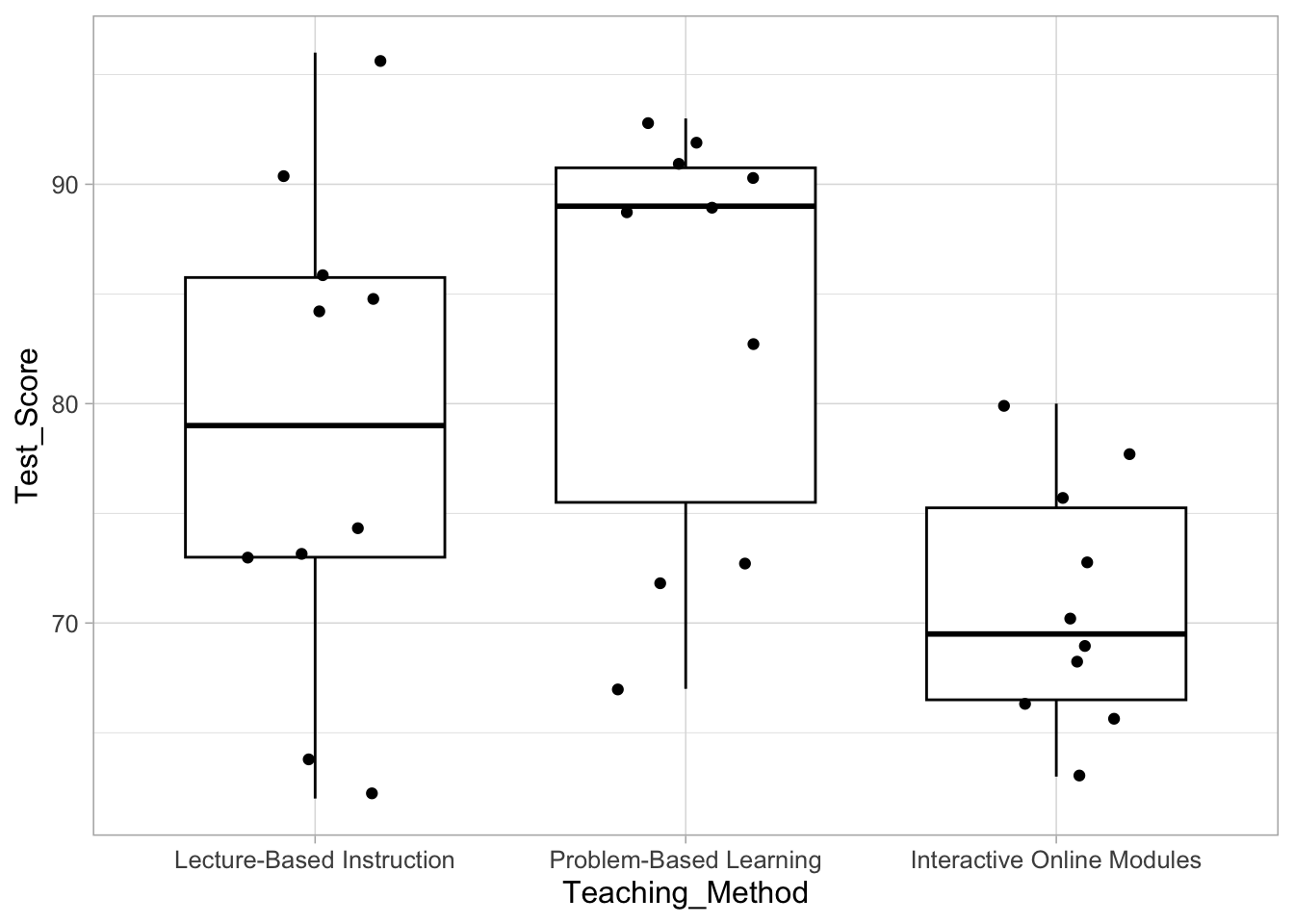
22.2.6.1 An Example

Imagine that a study is conducted to assess the impact of three different teaching methods (Lecture-Based Instruction, Problem-Based Learning, and Interactive Online Modules) on the academic performance of students in a statistics course. The study adopts a repeated measures design, where each student undergoes assessment under all three teaching methods. Student outcomes are then evaluated by measuring the number scores on a assessment test.

The following data are obtained:

Student_ID	Lecture-Based Instruction	Problem-Based Learning	Interactive Online Modules
1	90	83	66
2	74	91	69
3	73	89	68
4	62	92	78
5	96	89	63
6	73	73	73
7	84	93	76
8	85	67	70
9	86	72	66
10	64	90	80

Long-form

You can also conceptualize the data in ‘long’ form:

Student_ID	Teaching_Method	Test_Score
1	Lecture-Based Instruction	90
2	Lecture-Based Instruction	74
3	Lecture-Based Instruction	73
4	Lecture-Based Instruction	62
5	Lecture-Based Instruction	96
6	Lecture-Based Instruction	73
7	Lecture-Based Instruction	84
8	Lecture-Based Instruction	85
9	Lecture-Based Instruction	86
10	Lecture-Based Instruction	64
1	Problem-Based Learning	83
2	Problem-Based Learning	91
3	Problem-Based Learning	89
4	Problem-Based Learning	92
5	Problem-Based Learning	89
6	Problem-Based Learning	73
7	Problem-Based Learning	93
8	Problem-Based Learning	67
9	Problem-Based Learning	72
10	Problem-Based Learning	90
1	Interactive Online Modules	66
2	Interactive Online Modules	69
3	Interactive Online Modules	68
4	Interactive Online Modules	78
5	Interactive Online Modules	63
6	Interactive Online Modules	73
7	Interactive Online Modules	76
8	Interactive Online Modules	70
9	Interactive Online Modules	66
10	Interactive Online Modules	80

Let’s quickly visualize the data and get some descriptive statistics. Often, the median instead of mean are used for non-parametric tests.

Importantly, if the groups/conditions (IVs) have no true impact on participant outcomes (DVs), a participant would be equally likely to score their best on any condition. Furthermore, individuals ‘best’ ranking should even out at random across the conditions. For example, some people would score best in condition 1 (e.g., Lecture-Based Learning), while others would score best in condition 3 (e.g., Online). If we ranked within individuals across conditions, the ranking should even out and the sum of these rankings within conditions should be similar. It’s important to understand here that people are being rank within themselves and not in comparison to others.

Our first step will be to rank within individuals. So, if we recruited 10 individuals and had three experimental conditions, each participant would have a ranking of 1, 2, and 3. For our above data, we would get the following:

Original Data

Student_ID	Lecture-Based Instruction	Problem-Based Learning	Interactive Online Modules
1	90	83	66
2	74	91	69
3	73	89	68
4	62	92	78
5	96	89	63
6	73	73	73
7	84	93	76
8	85	67	70
9	86	72	66
10	64	90	80

New Data

Student_ID	Lecture-Based Instruction	Problem-Based Learning	Interactive Online Modules
1	1	2	3
2	2	1	3
3	2	1	3
4	3	1	2
5	1	2	3
6	2	2	2
7	2	1	3
8	1	3	2
9	1	2	3
10	3	1	2

Next we can calculate the sum of the ranks within each group.

Teaching_Method	Sum
Lecture-Based Instruction	18
Problem-Based Learning	16
Interactive Online Modules	26

Under the null, these sums should be similar. However, if are systematic differences, then groups should differ. In this case, teaching methods that seem to produce better results should have lower sums (e.g., more of people’s best/1st place rankings) compared to methods that produce poorer results (i.e., student’s ranked worse here).

We can use these rankings to now calculate our test statistic:

\(\chi_F^2 = \frac{12}{Nk(k+1)} ( \sum R_i^2 - 3N(k+1) )\)

• \(R_i\) = the sum of the ranks for the ith condition
• \(N\) = the number of participants
• \(K\) = the number of conditions

With \(k-1\) degrees of freedom.

22.2.6.2 Software

SPSS:

R:

`friedman.test(DV ~ IV | Grouping_Var, data=your_data)

Where:

• DV is your outcome (ranked or not)
• IV is your group/experimental conditions
• Grouping_Var are the participant IDs/blocks
• your_data is the name of your data frame

In our example:

• friedman_test(Test_Score~Teaching_Method |Student_ID, data=df_fried)

.y.	n	statistic	df	p	method
Test_Score	10	6.222222	2	0.04455143	Friedman test

22.2.6.3 Post-Hoc Analysis

The Friedman Test is an omnibus test, meaning it evaluates whether there are any statistically significant differences among three or more groups. However, to discern which specific groups exhibit significant differences, post-hoc tests are typically required.

One approach for post-hoc analysis involves conducting pairwise comparisons between groups. This can be achieved using Bonferroni- or Holm–adjusted Signed Rank Tests, which help identify specific group differences while controlling for multiple comparisons.

You can complete these post-hoc tests in R using the rstatix package.

your_data %>% 
  wilcox_test(DV ~ IV, paired=TRUE, p.adjust.method = 'bonferroni')

By replacing the above with your own data, IV, and DV. Note, changing paired=TRUE to paired=FALSE would conduct Rank Sums tests as opposed to Signed Rank tests.

For our data:

.y.	group1	group2	n1	n2	statistic	p	p.adj	p.adj.signif
Test_Score	Lecture-Based Instruction	Problem-Based Learning	10	10	14	0.343	1.000	ns
Test_Score	Lecture-Based Instruction	Interactive Online Modules	10	10	34	0.192	0.576	ns
Test_Score	Problem-Based Learning	Interactive Online Modules	10	10	44	0.013	0.038	*

Last, it is useful to visualize our data.

22.2.6.4 Effect Size

Measures such as Kendall’s W or the generalized eta-squared (\(\eta^2_g\)) are commonly used to quantify the magnitude of the differences observed among the related groups in the Friedman Test.

Kendall’s W

Kendall’s W is interpreted as the probability that two randomly selected measurements will have the same order in all groups. It ranges from 0 to 1, with larger values indicating a stronger effect. The higher the effect size, the more similar rankings are across times. It is calculated as:

For our data:

\(W = \frac{\chi^2_F}{N(K-1)}\)

\(W = \frac{6.222}{10(3-1)}=\frac{6.222}{20}=.3111\)

Or, in R:

friedman_effsize(DV ~ IV |ID, data = your_data)

Replacing with your data and variable names. For us, R would produce:

.y.	n	effsize	method	magnitude
Test_Score	10	0.3111111	Kendall W	moderate

22.2.6.5 Write-up

The Friedman test revealed a statistically significant difference in test scores across the three teaching methods, \(\chi^2_F(2) = 6.22, p=.044, W=.311\). Post-hoc Bonferroni-corrected signed rank tests were conducted to compare pairs of teaching methods. Student test scores when instructed in Lecture-Based Instruction (\(\sum_{rank}= 18\)) versus Problem-Based Instruction (\(\sum_{rank}= 16\)) were not statistically significantly different, \(V = 14, p >.999\). Additionally, Lecture-Based Instruction did not result in statistically significant test scores when compared to Online Instruction (\(\sum_{rank}= 26\)), \(V = 34, p = .576\). Last, Online Instruction did provide poorer and statistically significant test results compared to Problem-Based Instruction, \(V = 44, p = .038\).

22.2.6.6 Layperson Summary

In this study, researchers looked at three ways of teaching: lectures, problem-solving, and online lessons. They found that overall, there was a difference in how well students did on tests depending on the teaching method used. When they compared lectures to problem-solving, there wasn’t much of a difference in test scores. Also, lectures didn’t show much of a difference compared to online lessons. However, online lessons led to lower test scores compared to problem-solving. This suggests that problem-solving might be a better way to learn than online lessons. So, if given a choice, it’s probably a good idea to choose problem-based learning over online lessons.

22.3 Disadvantages to Non-parametrics

Until now, I have stated that non-parametric tests have an advantage over parametric tests because they do not rely on the distributional assumptions of parametrics– they are distribution free. However, there is a cost.

When working with data and research questions that permit the use of parametric tests, it makes sense to take this approach. That is, if you want to test the difference between two independent groups on continuous data, the independent t-test is likely a better option than a rank sum test. But why? What disadvantages are inherent in non-parametric tests.

Reduced Precision: Non-parametric methods, by their nature, often provide estimates that are less precise compared to parametric methods. This reduced precision stems from the fact that non-parametric approaches typically do not make assumptions about the underlying distribution of the data. Instead, they rely on ranking or other distribution-free techniques. As a result, the estimates produced by non-parametric methods may be more variable or less accurate than those obtained from parametric models, especially when the underlying distribution is well-understood and can be adequately described by a parametric form.

Less Efficient/Sample Size Sensitivity: Non-parametric methods generally require larger sample sizes to achieve comparable statistical power to parametric methods. In situations where sample sizes are limited, non-parametric methods may struggle to detect significant effects or accurately estimate parameters, making them less suitable for smaller datasets.

Difficulty in Interpretation: While non-parametric methods offer flexibility and robustness by not assuming specific distributions, they can be more challenging to interpret. Parametric models often provide explicit parameter estimates that are easily interpretable in the context of the research question. For example, \(R^2\) as the proportion of variance accounted for or Cohen’s D being a standardized mean different between two groups. In contrast, non-parametric methods may produce results that are more abstract or less straightforward to interpret. This can be challenging for researchers in drawing meaningful conclusions from their analyses. In turn, this will make it difficult for others to understand and interpret the results.

22.4 Conclusion

Non-parametric are useful statistical tools for you to have. They have the benefit of not relying on many of the assumptions of parametric tests. We explored several major non-parametric “siblings” to parametric tests you are familiar with. By having these tools available, you can expand the types of research questions you can answer (e.g., those with ordinal variables) and overcome issues that may pop up in your research (e.g., violation of assumptions). However, these tests should be interpreted within the context of their limitations or disadvantages.