| Bag | Store | Weight |
|---|---|---|
| 1 | Wilsons | 201.067 |
| 2 | Wilsons | 191.670 |
| 3 | Myles | 194.584 |
| 4 | Myles | 191.286 |
| 5 | Colemans | 189.917 |
| 6 | Colemans | 194.987 |
8 z-test
:max_bytes(150000):strip_icc()/73135-homestyle-potato-chips-ddmfs-0348-3x4-hero-c21021303c8849bbb40c1007bfa9af6e.jpg)
This chapter will cover the z-test. Although more details follow, in short, a z-test is a statistical method used to determine if there is a significant difference between a sample mean and a known population mean assuming the population variance is known. It calculates a z-score, which measures how many standard deviations the sample mean is from the population mean. By comparing this z-score to a critical value from the standard normal distribution, researchers can determine whether the observed difference is statistically significant. These tests are commonly used in large-sample studies where population parameters are available.
8.1 Betcha’ can’t eat just one!
Imagine we wanted to model the average weight of a bag of Lay’s Potato Chips. Let’s use our scientific method, as discussed in an earlier chapter, to conduct some science.
Specifically, you have a theory that, despite being listed as 200g, the large bag of chips actually weighs less because the company cuts corners to save money and is, thus, dishonest about the weight. So you hypothesize that Lays chips that are listed as 200g do not weigh 200g.
- Generate your hypotheses:
Our hypothesis that “Lays chips that are listed as 200g do not weigh 200g” can be translated into a statistical hypothesis, which is represented as the null and alternative hypotheses:
\(H_0: \mu_{lays}=200g\)
\(H_1: \mu_{lays}<200g\)
You email Lays and they respond, indicating that their chips, on average, weight 200g, but have some variability. Specifically, they say the standard deviation of weight of the chips is 6g. You aren’t satisfied with that response and continue with your research.
It is impossible for you to weigh every produced ‘200g’ bag of Lays chips, so you decide to take a sample. You decide to use NHST to test the weights of bags and use a \(\alpha=.05\) criterion.
- Designing a study
You plan a study wherein you will drive around Corner Brook to three popular stores: Sobey’s, Myles’s, and Coleman’s. You will buy two 200g bags of Lays at each location, resulting in a total sample size of six (n = 6). Once you have the chips, you will bring them to your home and weigh them on a professionally calibrated weight scale. You decide to pour the chips out of the bag, as Lay’s communicated that the weight indicates the chips put in a bag and does not include the bag.
Additionally, you submit your research plan to the Grenfell Campus research ethics board. They foresee no risks and allow you to complete the study.
- Collecting data
You follow through with your research plan. You get the following data:
- Analyzing data
We know the population mean (\(\mu=200\)) and standard deviation (\(\sigma=6\)). Let’s calculate our sample mean and standard deviation.
| Mean | SD |
|---|---|
| 193.9185 | 4.01705 |
8.1.1 Mean, Standard Deviation, and Variance
Remember, the mean is a measure of central tendency and is (here, population):
\(\mu = \frac{\sum_{i=1}^{n} x_{i}}{n}\)
and population standard deviation is:
\(\sigma = \sqrt{\frac{\sum_{i=1}^N (x_i - \overline{x})^2}{N}}\)
and population variance is:
\(\sigma^2 = \frac{\sum_{i=1}^N (x_i - \overline{x})^2}{N}\)
You may remember that the population and sample standard deviation differ in the denominator. The sample SD and variance have \(n-1\) as a denominator versus the population’s \(n\). Why?
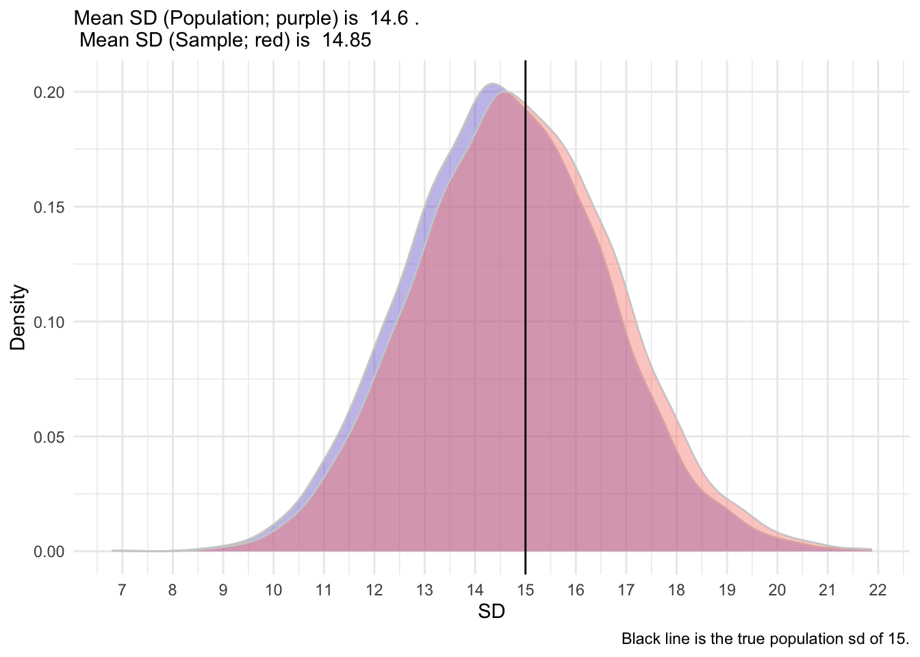
Standard deviations are typically biased downward (they underestimate the true standard deviation), so the \(n-1\) makes is less biased. Let’s take an example. Consider a population with a mean of 100 and standard deviation of 15.
Let’s take a sample of 30 people from that population and calculate the standard deviation. We get the following SD:
[1] 11.91149So, because it’s an estimate, it has some degree of error. It’s not expected to be exactly 15. But what it we took 5000 samples?
After I simulated 5,000 sample, I get the following distribution of SD.

So, as you can see, the sample formula provides a less biased estimate of the true population SD. It’s shifted slightly to the right, closer to the true population SD. We hope that the mean and standard deviation that we collect in a sample (termed statistics) are somewhat good indicators of those in the population (termed parameters).
Calculate the mean, sample SD, and sample variance of the following two variables, x and y:
| x | y |
|---|---|
| 6 | 10 |
| 3 | 6 |
| 12 | 8 |
| 3 | 9 |
| 6 | 4 |
| Mean_x | SD_x | Mean_y | SD_y |
|---|---|---|---|
| 6 | 3.674235 | 7.4 | 2.408319 |
8.1.2 Visualizing Chips
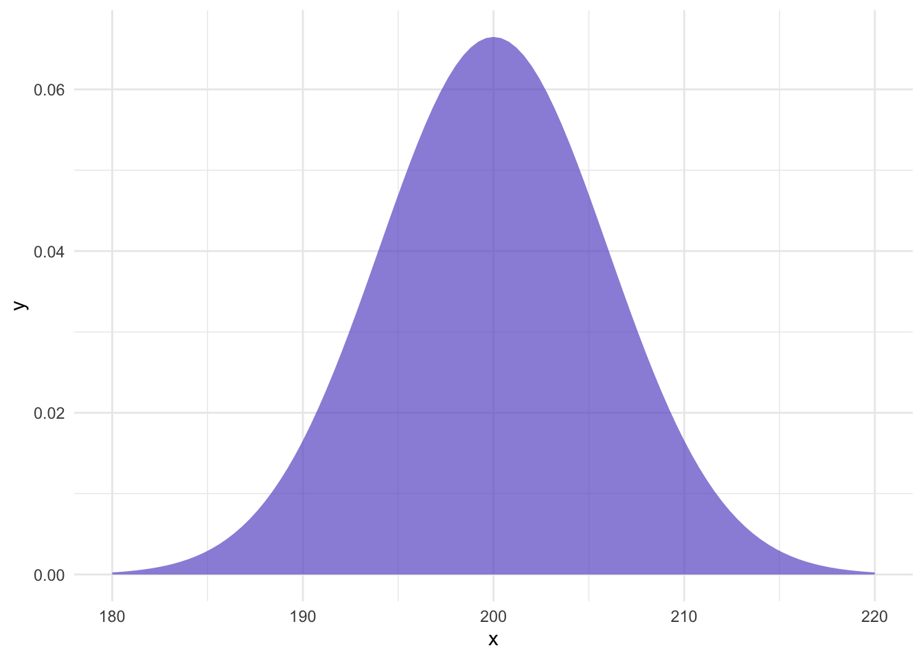
Given that Lays has communicated the population parameters, we can calculate how likely our sample is. First, let’s visualize the distribution of chips with a \(\mu=200\) and \(\sigma=6\):

When we repeatedly take samples from a population and calculate the mean of each sample, the distribution of these sample means forms what’s known as the sampling distribution of the sample mean.
Importantly, according to the Central Limit Theorem (CLT), no matter what the original distribution of the data looks like (as long as it has a finite mean and variance), the sampling distribution of the sample mean will tend to be normally distributed as the number of samples increases. This is true even if the population distribution is not normal.
The mean of the sampling distribution of the sample mean (often denoted \(\mu_{\bar{x}}\)) will be the same as the mean of the original population. So if the average weight of chip bags in the population is, say, 200 grams, then the mean of all those sample means will also be 200 grams.
The standard deviation of the sampling distribution (called the standard error) is smaller than the population standard deviation. It is calculated as:
\(\text{Standard Error} = \frac{\sigma}{\sqrt{n}}\)
Where \(\sigma\) is the population standard deviation and \(n\) is the sample size. This means that the variability (spread) of the sample means is less than the variability of individual data points in the population. Additionally, as the sample size increases, the standard error approaches 0. That is, a larger sample size provides a more precise estimate of the population mean.
If you plot the means of all these samples of 6 bags, you would get a normal-shaped bell curve (assuming you’ve taken a large number of samples), with the peak centered at the population mean. The spread (or width) of this bell curve depends on the sample size and population standard deviation. The more samples you take, the smoother and more normal the distribution of sample means will look.
In our example, if we take a sample of six bags, calculate the average weight of those six bags, and repeat this process many times, we would end up with a collection of sample means.

As you can see from the figure, when you collect the mean of six random bags of chips many times, they form another normal distribution.
Standard Error
The standard error is the standard deviation of sample means. A large standard error indicates high variability between the means of different samples. Therefore, your sample may not be a good representation of the true population mean. This is not good.
A small standard error indicates low variability between the means of different samples. Therefore, our sample mean is likely reflective of the population mean. This is good.
Step 4: Analyse
8.2 z-test
Should the above distribution of sample means truly follow a normal distribution, then we should be able to calculate how likely our sample of six bag of chips is! We can fill in the what we know, according to Lays: \(\mu_{\bar{x}} = \mu = 200\) and; \(\sigma_{\bar{x}} = \frac{\sigma}{\sqrt{n}} = \frac{6}{\sqrt{6}} = 2.4495\).
So, the probability of getting our sample mean of 193.92 can be converted into a z-score:
\(z = \frac{x - \bar{x}}{\sigma_{\bar{x}}} = \frac{193.9185 - 200}{2.4495} = -2.482752\)
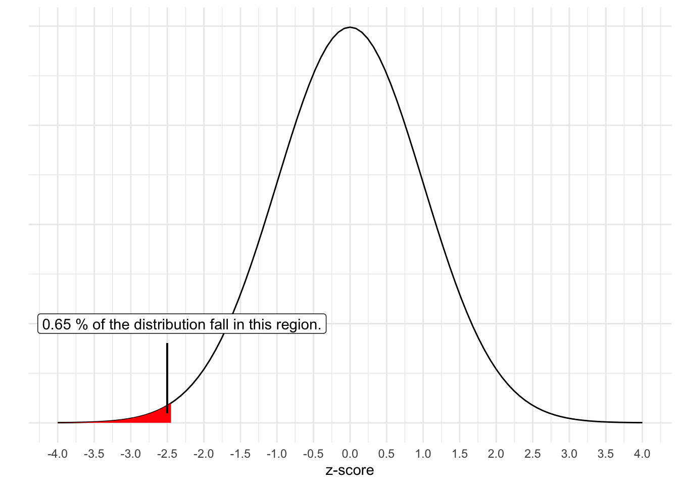
Additionally, the probability of getting a z-score that low is 0.0065. Recall that the normal distribution has some unique properties and we can find out the proportion of scores that fall in the tails. While you may have used table like the previous link in past courses, computers can easily determine the exact quantity (e.g., pnorm() in R).

Hypothetically, out of 1000 samples of six bags of chips drawn from the distribution of \(\mu=200\) and \(\sigma=6\), we would get a score as low as our sample mean or lower less than 7 times. Our sample is very unlikely if Lays is telling the truth!
You just did a z-test. Let’s run it in R to ensure we get the same numbers! Recall our data:
| Bag | Store | Weight |
|---|---|---|
| 1 | Wilsons | 201.067 |
| 2 | Wilsons | 191.670 |
| 3 | Myles | 194.584 |
| 4 | Myles | 191.286 |
| 5 | Colemans | 189.917 |
| 6 | Colemans | 194.987 |
The assumption is that we have randomly sampled. That is:
\(H_{0}: \mu = 200\);
and
\(H_{1}: \mu < 200\).
What would you conclude from the following output?
Step 5: Write up your results/conclusions
When interpreting this, we can say that the likelihood of getting our sample mean of 193.91 or lower is unlikely given a true null hypothesis that \(\mu=200\), z = -2.48, p = .0065. This is referred to as statistical significance.
8.3 Conclusion
A z-test is a statistical method used to determine if there is a significant difference between a sample mean and a known population mean assuming the population variance is known. It calculates a z-score, which measures how many standard deviations the sample mean is from the population mean. By comparing this z-score to a critical value from the standard normal distribution, researchers can determine whether the observed difference is statistically significant. These tests are commonly used in large-sample studies where population parameters are available.
Building your toolbox. After each analytic tool, we will begin to add to a table that provides brief details about the tool. You can then refer back to this at a later time when conducting your own research.
| Name | Uses | Number of IVs | Number of DVs | IV | DV | Assumptions | Hypotheses | Effect Size |
|---|---|---|---|---|---|---|---|---|
| z-test | Compare one group's mean to a population mean. | 0 (No IVs) | 1 | None or Categorical (e.g., Group) | Continuous | Normality, known population variance | Null: Mean of group equals population mean, Alternative: Mean of group differs from population mean | Cohen's d |
What’s the difference is the probability of sampling a single bag of chips weighting 190g in a sample versus getting a mean weight of 190g for 10 bags of chips? Why are they different? How to the distributions differ?
What happens to the SD of the distribution of sample means as the sample size increases? Imagine drawing 100,000 bags of chips.
Suppose a university claims that the average score on a standardized test for psychology students is 75 with a standard deviation of 10. We collect a sample of 15 students’ test scores to see if the average score differs from 75. The following are the scores:
| Person | Score |
|---|---|
| 1 | 78 |
| 2 | 74 |
| 3 | 61 |
| 4 | 75 |
| 5 | 57 |
| 6 | 80 |
| 7 | 82 |
| 8 | 66 |
| 9 | 74 |
| 10 | 90 |
| 11 | 81 |
| 12 | 64 |
| 13 | 52 |
| 14 | 45 |
| 15 | 87 |
- What is the sample mean?
- Perform a one-sample z-test: Is the sample mean significantly different from the claimed population mean of 75? Use a population standard deviation of 10 and a significance level of 0.05.
- What is the z-score for this test?
- What is the p-value for the z-test? Does it allow us to reject the null hypothesis?
