| track_artist | track_name | Popularity | Valence | Danceability |
|---|---|---|---|---|
| Camila Cabello | My Oh My (feat. DaBaby) | 208 | 13 | 2 |
| Tyga | Ayy Macarena | 95 | 17 | 7 |
| Maroon 5 | Memories | 200 | 23 | 4 |
| Harry Styles | Adore You | 62 | 9 | 9 |
| Sam Smith | How Do You Sleep? | 189 | 22 | 4 |
| Tones and I | Dance Monkey | 87 | 19 | 7 |
| Lil Uzi Vert | Futsal Shuffle 2020 | 140 | 1 | 5 |
| J Balvin | LA CANCIÓN | 144 | 14 | 5 |
| Billie Eilish | bad guy | 129 | 6 | 7 |
| Dan + Shay | 10,000 Hours (with Justin Bieber) | 141 | 8 | 5 |
| Regard | Ride It | 191 | 13 | 3 |
| Billie Eilish | bad guy | 175 | 19 | 5 |
| The Weeknd | Heartless | 126 | 13 | 4 |
| Y2K | Lalala | 112 | 18 | 5 |
| Future | Life Is Good (feat. Drake) | 36 | 16 | 8 |
| Lewis Capaldi | Someone You Loved | 76 | 17 | 6 |
| Anuel AA | China | 185 | 22 | 4 |
| Regard | Ride It | 162 | 17 | 5 |
| Dua Lipa | Don't Start Now | 144 | 7 | 4 |
| Anuel AA | China | 144 | 12 | 5 |
| Regard | Ride It | 133 | 13 | 5 |
| Bad Bunny | Vete | 107 | 13 | 6 |
| Roddy Ricch | The Box | 142 | 7 | 2 |
| Juice WRLD | Bandit (with YoungBoy Never Broke Again) | 109 | 12 | 7 |
| Roddy Ricch | The Box | 247 | 25 | 4 |
| Regard | Ride It | 133 | 14 | 5 |
| Trevor Daniel | Falling | 149 | 11 | 4 |
| Anuel AA | China | 190 | 15 | 3 |
| Shawn Mendes | Señorita | 140 | 8 | 4 |
| Travis Scott | HIGHEST IN THE ROOM | 186 | 10 | 3 |
| Juice WRLD | Bandit (with YoungBoy Never Broke Again) | 164 | 21 | 4 |
| Camila Cabello | My Oh My (feat. DaBaby) | 135 | 22 | 6 |
| Sam Smith | How Do You Sleep? | 113 | 12 | 5 |
| Harry Styles | Adore You | 129 | 10 | 4 |
| Don Toliver | No Idea | 53 | 20 | 7 |
| Billie Eilish | everything i wanted | 133 | 20 | 5 |
| Lil Uzi Vert | Futsal Shuffle 2020 | 65 | 21 | 7 |
| DaBaby | BOP | 111 | 16 | 5 |
| Lil Uzi Vert | Futsal Shuffle 2020 | 18 | 23 | 8 |
| blackbear | hot girl bummer | 166 | 17 | 4 |
| Tones and I | Dance Monkey | 198 | 13 | 2 |
| Tyga | Ayy Macarena | 87 | 13 | 6 |
| Selena Gomez | Lose You To Love Me | 113 | 11 | 5 |
| Dalex | Hola - Remix | 106 | 15 | 5 |
| The Black Eyed Peas | RITMO (Bad Boys For Life) | 100 | 11 | 8 |
| Arizona Zervas | ROXANNE | 116 | 11 | 6 |
| The Black Eyed Peas | RITMO (Bad Boys For Life) | 111 | 4 | 6 |
| Arizona Zervas | ROXANNE | 101 | 14 | 6 |
| Roddy Ricch | The Box | 57 | 13 | 8 |
| MEDUZA | Lose Control | 119 | 23 | 6 |
18 Multiple Regression
This chapter will cover multiple regression, a statistical method used to examine the relationship between a dependent (or outcome/criterion) variable and multiple independent (predictor) variables. Unlike simple regression, which involves only one predictor, multiple regression allows researchers to assess the combined influence of several predictors on an outcome. But why do researchers need multiple predictors?
Using multiple predictors in regression allows researchers to better understand complex relationships between variables. Real-world outcomes are rarely influenced by a single factor; instead, they result from multiple interacting influences. By including multiple predictors, we can control for confounding variables, improve the accuracy of our predictions, and gain a more comprehensive understanding of how different factors contribute to an outcome.
18.1 Some Additional Details
Multiple regression is useful in situations where we expect multiple factors to influence an outcome. For example, a researcher might want to predict job performance based on cognitive ability, motivation, and job experience.
The general form of the multiple regression equation is:
\[ y_i = \beta_0 + \beta_1x_1 + \beta_2x_2 + ... + \beta_nx_n + e_i \]
where:
- \(Y\) is the dependent variable (outcome of interest),
- \(X_1, X_2, ..., X_n\) are independent variables (predictors),
- \(\beta_0\) is the intercept (value of \(Y\) when all predictors are 0),
- \(\beta_1, \beta_2, ..., \beta_n\) are regression coefficients representing the effect of each predictor on \(Y\),
- \(e\) is the error term.
18.1.1 Key Assumptions
Like all of our analyses thus far, a multiple regression analysis is valid model under the following assumptions (many we have already explored):
1. Linearity
The relationship between each predictor and the dependent variable should be linear.
2. Independence of Errors
Observations should be independent, and errors should not be correlated.
3. Homoscedasticity
The variance of errors should be constant across all levels of the independent variables.
4. Normality of Residuals
The residuals (errors) should be normally distributed.
5. No Multicollinearity
Predictor variables should not be highly correlated with one another. More to come.
Prior to further exploring our hypotheses and conducting a formal analysis, an explanation of various types of correlations is needed. Correlations help us understand the relationships between variables and are particularly important in multiple regression, where we assess the contribution of multiple predictors to an outcome variable.
18.2 Types of Correlations
18.2.1 Pearson Correlation Coefficient
We have already explored correlation, \(r\), in a previous chapter. Recall that when we square the correlation, we obtain the coefficient of determination (\(R^2\)), which indicates the proportion of variance in one variable that is accounted for/explained by (not to be confused with CAUSED BY) the other. This provides insight into how strongly two variables are related, but it does not imply causality. Recall that one formula for the Pearson correlation coefficient is:
\[ r = \frac{\sum (X_i - \bar{X})(Y_i - \bar{Y})}{\sqrt{\sum (X_i - \bar{X})^2 \sum (Y_i - \bar{Y})^2}} \]
where:
- \(X_i\) and \(Y_i\) are individual data points,
- \(\bar{X}\) and \(\bar{Y}\) are the means of the variables,
- The numerator represents the covariance between \(X\) and \(Y\),
- The denominator standardizes the covariance by dividing by the product of the standard deviations.
To visualize the coefficient of determination, consider the following two variables: \(x_1\) and \(y\).
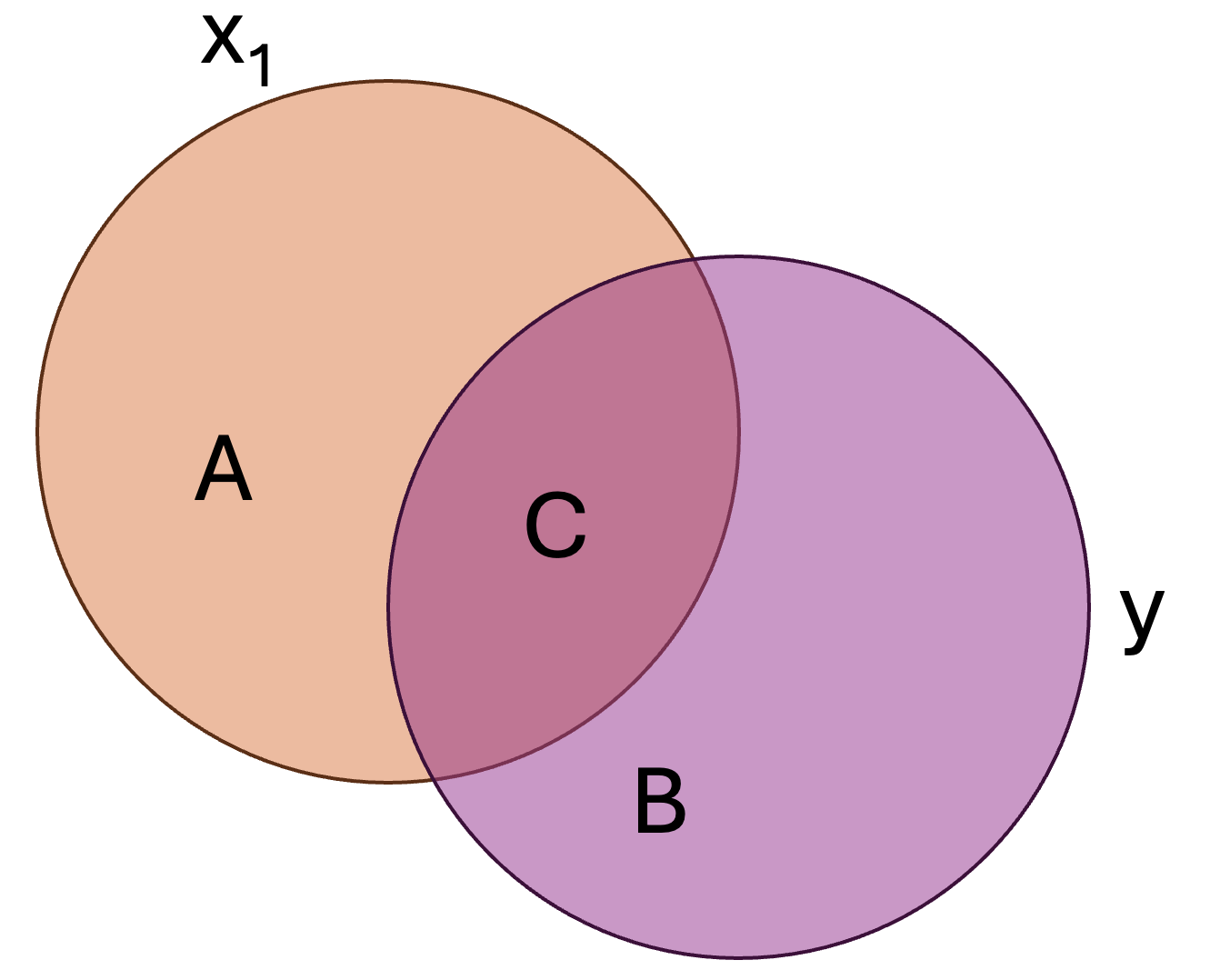
Here:
- \(B + C\) represents the total variance in \(y\), or \(\sigma^2_y\)
- \(C\) represents the variance in \(y\) that is accounted for/explained by \(x_1\), or \(R^2\)
- \(B\) represents the variance that is unaccounted for in the model
18.2.2 Semi-Partial Correlation (Part Correlation)
The semi-partial correlation, denoted as \(r_{x1(y.x2)}\) (where we have three variables: \(x_1\), \(x_2\), and \(y\)), measures the unique relationship between one predictor and the outcome variable after controlling for the effects of another predictor on that predictor (but not on the outcome variable). This is particularly useful when we want to understand how much unique variance a predictor contributes to the dependent variable without adjusting for other predictors’ influence on the outcome.
For example, if we are examining the relationship between study hours (\(x_1\)) and exam scores (\(y\)), while controlling for prior GPA (\(x_3\)), the semi-partial correlation tells us how much variance in exam scores is uniquely explained by study hours that is not shared with prior GPA.
In short, it is the variance uniquely explained relative to all of criterion. Let’s not visualize this regression model, wherein we have two predictors, \(x_1\) and \(x_2\), predicting the criterion, \(y\):
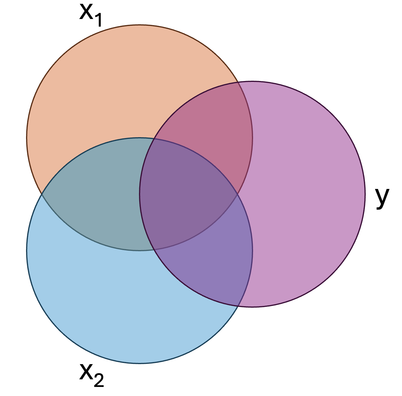
We can assign each region of the above figure a letter:
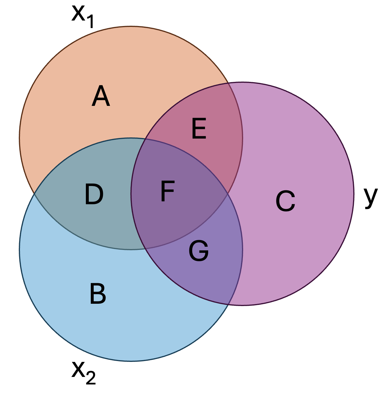
In this figure:
- \(E+F+G+C\) represents the total variance in \(y\), or \(\sigma^2_y\)
- \(E+F+G\) represents the total variance explained by the model, or \(R^2\)
- \(C\) represents the unaccounted for/unexplained variance in \(y\), or \(1-R^2\)
- \(E+F\) represents the total variance in \(y\) explained by \(x_1\), or \(r^2_{x_1y}\)
- \(E\) represents the unique variance in \(y\) explained by \(x_1\)
- \(F+G\) represents the total variance in \(y\) explained by \(x_2\), or \(r^2_{x_2y}\)
- \(G\) represents the unique variance in \(y\) explained by \(x_2\)
- \(F\) represents the shared variance in \(y\) explained by \(x_1\) and \(x_2\)
In the regular Pearson correlation, \(E+F\) would have been considered the variance in \(y\) explained by \(x_1\). However, some of this variance is also explained by \(x_2\). One way to represent this is by the squared semi-partial or part correlation (note: we are squaring it to give us the ‘proportion of variance’, just as we did in correlation). The squared semi-partial/part correlation of \(x_1\) and \(y\) would be:
\[ r_{x_1(y.x_2)}^2=\frac{E}{C+E+F+G} \]
Or, simply:
\[ r_{x_1(y.x_2)}^2=R^2-r^2_{x_2y} \]
In the above formula we are, essentially, saying that \(r^2_{x_1(y.x_2)}\) is the difference between \(R^2\), the total variance in \(y\) and \(r^2_{x2y}\), the total variance in \(y\) explained by \(x_2\). Logically, this means that in this two predictor model, any variance in \(y\) that is not explain by \(x_2\) is uniquely explained by \(x_1\). Note the differences in the notation between the Pearson correlation between the two, \(r_{x_1y}\), and the part correlation that accounts for \(x2\), \(r_{x_1(y.x_2)}\).
Practice
- What regions would represent the squared semi-partial/part correlation of \(x_2\) and \(y\)?
- What would be the mathematical formula?
Click to reveal answers
\(r_{x_2(y.x_1)}^2=\frac{G}{C+E+F+G}\)
\(r_{x_2(y.x_1)}^2=R^2-r^2_{x_1y}\)
18.2.3 Partial Correlation
The partial correlation, denoted as or \(r_{x1y.x_2}\), assesses the direct relationship between a predictor and the outcome variable after controlling for the influence of other predictors on both the predictor and the outcome. This differs from the semi-partial correlation because it removes the effect of control variables or other predictors (in our above example, \(x_2\)) from both the predictor of interest and the outcome.
Mathematically, the squared partial correlation, \(r_{x1y.x_2}^2\), tells us the proportion of variance in \(y\) that is uniquely explained by \(x_1\) after removing the influence of all other predictors. In short, it is the variance uniquely explained relative to the unexplained variance of the criterion.
The squared partial correlation of \(x_1\) and \(y\) would be:
\[ r_{x_1y.x_2}^2=\frac{E}{C+E} \]
Or, mathematically:
\[ r_{x_1y.x_2}^2=\frac{R^2-r^2_{x_2y}}{1-r^2_{x_2y}} \]
Both partial and semi-partial correlations help us understand how an independent variable (IV) relates to the dependent variable (DV) while accounting for other variables in a regression model. However, they answer slightly different questions. Here is a quick reference to help you.
1. Partial Correlation → “What is the pure relationship between this predictor and the outcome?”
- It tells you how much an IV is related to the DV after removing the influence of other IVs from both the predictor and the outcome.
- Example: If you’re studying how stress affects exam scores while controlling for sleep, the partial correlation tells you the direct relationship between stress and scores as if sleep was completely removed from the equation for both stress and scores.
2. Semi-Partial (Part) Correlation → “How much does this predictor add to the model’s ability to predict the outcome?”
- It tells you how much an IV uniquely contributes to explaining the DV without adjusting the DV itself.
- Example: If you add stress as a predictor to your exam scores model (which already includes sleep), the semi-partial correlation tells you how much extra variance in exam scores is explained just by stress (after removing overlap with sleep in stress but not in the scores).
In this class we will primarily use the semi-partial/part correlation–mostly the squared part correlation–in our regression analyses. With this in mind, let’s continue with a practical example involving our favorite musician, Taylor Swift.
18.3 Regression…you can do it with a broken heart.
Taylor Swift and her team are consulting you, a research expert, to help determine what features of music determine the popularity it achieves. She hopes to use your findings to write new music. Specifically, she is interested in knowing whether certain characteristics of music are more likely to get played on Spotify. Taylor and her team have a theory that they have called the “Rhythmic Positivity Theory”. This proposes that songs with higher danceability and happier tones are more popular because they elicit positive emotions and encourage social engagement. Taylor also has specific hypotheses: that both both positively valenced (i.e., happy) and danceable songs will be more popular.
18.4 Step 1. Generate your hypotheses
In regression you hypothesize about coefficients, typically referred to as \(\beta\)s (beta), or the full model. Thus, we could have two different sets of hypotheses. The most common will refer to coefficients. Here, we could convert our text-based hypotheses to statistical hypotheses:
\(H_0:\beta_{dance}=0\) and \(\beta_{valence}=0\)
and
\(H_A:\beta_{dance}\ne0\) and \(\beta_{valence}\ne0\)
We will use \(\ne\) for these alternative hypotheses because they could be positive or negative and we are doing a two-tailed test. The second type of hypotheses we may propose have to do with the full model, and how well it accounts for variance in the outcome (i.e., DV/criterion):
\[ H_0:R^2=0 \]
\[ H_A:R^2>0 \]
We use \(>\) for this hypothesis because \(R^2\) cannot be negative.
While these are our main hypotheses, we should also try to conceptualize our study’s model. Our model can be represented as follows:
\[ y_i=\beta_0+\beta_{dance}(x_{dance,i})+\beta_{valence}(x_{valence,i})+e_i \]
Where \(x_{dance,i}\) is individual \(i\)’s score on danceability, \(x_{valence,i}\) is individual \(i\)’s score on valence \(\beta_0\) is the intercept of the model, \(\beta_{dance}\) is the coefficient for danceability and \(\beta_{valence}\) is the coefficient for valence. Last, \(e_i\) is the error for individual i.
18.5 Step 2. Designing a study
While Taylor has given you a $3,000,000 budget, you decide to put that money in you RRSP, cheap out, and collect publically-available data from Spotify. You decide that you will collect a random sample of songs from Spotify and use a computer to estimate the valence and danceability of the songs. These are both measured as continuous variables. You decide to use a regression to determine the effects of both variables on a song’s popularity (number of plays on Spotify in 2023, in millions). All variables are continuous (although regression can handle most variable types; ANOVA is just a special case of regression).
You do a power analysis and determine you need a sample of approximately 50 songs.Prior to conducting your research, you submit your research plan to the Grenfell Campus research ethics board, which approves your study and classified it as low-risk.
18.6 Step 3. Conducting your study
You follow through with your research plan and get the following data:
Our Data
18.7 Step 4. Analyzing your data.
Matrix Algebra
Matrix algebra can be used to ‘solve’ our regression equation. However, we will not use matrix algebra to solve our regression coefficients in this class. For those interested, we could using the following (see here for more information):
\((X^′X)^{−1}X^′Y\)
Where \(X\) is a \(n\) by \(v\) matrix of scores, where n is the number of observations and v is the number of IVs (note: the first column will be 1s to represent the link to the intercept). \(Y\) is a \(n\) by \(1\) vector of scores on the DV.
Here, X is:
\[\begin{bmatrix} 1.00 & 13.00 & 2.00 \\ 1.00 & 17.00 & 7.00 \\ 1.00 & 23.00 & 4.00 \\ 1.00 & 9.00 & 9.00 \\ 1.00 & 22.00 & 4.00 \\ 1.00 & 19.00 & 7.00 \\ 1.00 & 1.00 & 5.00 \\ 1.00 & 14.00 & 5.00 \\ 1.00 & 6.00 & 7.00 \\ 1.00 & 8.00 & 5.00 \\ 1.00 & 13.00 & 3.00 \\ 1.00 & 19.00 & 5.00 \\ 1.00 & 13.00 & 4.00 \\ 1.00 & 18.00 & 5.00 \\ 1.00 & 16.00 & 8.00 \\ 1.00 & 17.00 & 6.00 \\ 1.00 & 22.00 & 4.00 \\ 1.00 & 17.00 & 5.00 \\ 1.00 & 7.00 & 4.00 \\ 1.00 & 12.00 & 5.00 \\ 1.00 & 13.00 & 5.00 \\ 1.00 & 13.00 & 6.00 \\ 1.00 & 7.00 & 2.00 \\ 1.00 & 12.00 & 7.00 \\ 1.00 & 25.00 & 4.00 \\ 1.00 & 14.00 & 5.00 \\ 1.00 & 11.00 & 4.00 \\ 1.00 & 15.00 & 3.00 \\ 1.00 & 8.00 & 4.00 \\ 1.00 & 10.00 & 3.00 \\ 1.00 & 21.00 & 4.00 \\ 1.00 & 22.00 & 6.00 \\ 1.00 & 12.00 & 5.00 \\ 1.00 & 10.00 & 4.00 \\ 1.00 & 20.00 & 7.00 \\ 1.00 & 20.00 & 5.00 \\ 1.00 & 21.00 & 7.00 \\ 1.00 & 16.00 & 5.00 \\ 1.00 & 23.00 & 8.00 \\ 1.00 & 17.00 & 4.00 \\ 1.00 & 13.00 & 2.00 \\ 1.00 & 13.00 & 6.00 \\ 1.00 & 11.00 & 5.00 \\ 1.00 & 15.00 & 5.00 \\ 1.00 & 11.00 & 8.00 \\ 1.00 & 11.00 & 6.00 \\ 1.00 & 4.00 & 6.00 \\ 1.00 & 14.00 & 6.00 \\ 1.00 & 13.00 & 8.00 \\ 1.00 & 23.00 & 6.00 \\ \end{bmatrix}\]And Y is:
\[\begin{bmatrix} 208.00 \\ 95.00 \\ 200.00 \\ 62.00 \\ 189.00 \\ 87.00 \\ 140.00 \\ 144.00 \\ 129.00 \\ 141.00 \\ 191.00 \\ 175.00 \\ 126.00 \\ 112.00 \\ 36.00 \\ 76.00 \\ 185.00 \\ 162.00 \\ 144.00 \\ 144.00 \\ 133.00 \\ 107.00 \\ 142.00 \\ 109.00 \\ 247.00 \\ 133.00 \\ 149.00 \\ 190.00 \\ 140.00 \\ 186.00 \\ 164.00 \\ 135.00 \\ 113.00 \\ 129.00 \\ 53.00 \\ 133.00 \\ 65.00 \\ 111.00 \\ 18.00 \\ 166.00 \\ 198.00 \\ 87.00 \\ 113.00 \\ 106.00 \\ 100.00 \\ 116.00 \\ 111.00 \\ 101.00 \\ 57.00 \\ 119.00 \\ \end{bmatrix}\]The results would work out to:
\[\begin{bmatrix} 237.42 \\ 1.09 \\ -23.79 \\ \end{bmatrix}\]Where each row is \(\beta_0\) to \(\beta_3\). Thus, the equation would be:
\[ y_i=237.42+1.09(x_{valence,i})+(-23.79)(x_{dance,i})+e_i \]
When we had one variable, we could effectively visualize a line of best fit. We can visualize a ‘plane’ of best fit when we have two predictors. For example, our data is represented as (you should be able to rotate this figure!):
As we now have more variables, the visualization becomes difficult. We struggle to interpret anything beyond 3D!
18.8 SST
Like simple regression, sum of squares total (SST) represents the difference between the observed scores on the outcome/criterion and the mean of the outcome/criterion.
\[ SST=\sum(y_i-\overline{y})^2 \]
18.9 SSE
Like simple regression, the sum of squares error/residual (SSE) represents the difference between the observed scores on the outcome/criterion and the predicted values of the outcome/criterion.
\[ SSR=\sum(y_i-\hat{y_i})^2 \]
18.10 SSR
Like simple regression, the sum of suqares regression/model (SSR) represents the difference between the predicted values on the outcome/criterion and the mean of the outcome/criterion
\[ SSM=\sum(\hat{y_i}-\overline{y})^2 \]
Although the main R output does not provide the sums of squares for our model, knowing the above allows you to manually calculate them. For us:
[1] "SSE = 33118.68. SSR = 74669.74. SST = 107788.42."Given these, we can calculate the MSR (mean square of the regression; with \(p-1\) degrees of freedom; p being the number of \(b\) coefficients) and MSE (mean square error; with \(n-p\) degrees of freedom) and calculate the appropriate F-statistic.
\[ MSR=\frac{74669.74}{2}=37334.87 \]
and
\[ MSE=\frac{33118.68}{47}=704.65 \]
and
\[ F=\frac{MSR}{MSE}=\frac{37334.87}{704.65}=52.98 \]
And you can look up the associated p-value in any standard critical F table. Or R can calculate it for us using pf(q=52.98, df1=2, df2=47) (the probability of F with our given).
18.10.1 \(R^2\)
Like simple regression, we can calculate an effect size (\(R^2\)). We can calculate this using:
\[ R^2=1-\frac{SSE}{SST}=\frac{33118.68}{107788.42}=.69 \]
18.10.2 Formal Analysis
There are multiple ways we can run a regression in R. We will use the basic lm() function that we used in the simple regression chapter.
taylors_model <- lm(Popularity ~ Valence +Danceability, data=taylor)and the summary of that model:
| Observations | 50 |
| Dependent variable | Popularity |
| Type | OLS linear regression |
| F(2,47) | 52.98 |
| R² | 0.69 |
| Adj. R² | 0.68 |
| Est. | S.E. | t val. | p | |
|---|---|---|---|---|
| (Intercept) | 237.42 | 15.61 | 15.21 | 0.00 |
| Valence | 1.09 | 0.70 | 1.56 | 0.13 |
| Danceability | -23.79 | 2.32 | -10.26 | 0.00 |
| Standard errors: OLS |
Also recall that the apaTables() package provides some additional information that is useful for our interpretation.
Regression results using Popularity as the criterion


    Predictor        b         b_95%_CI  beta    beta_95%_CI sr2  sr2_95%_CI
  (Intercept) 237.42** [206.02, 268.83]
      Valence     1.09    [-0.32, 2.50]  0.13  [-0.04, 0.29] .02 [-.02, .05]
 Danceability -23.79** [-28.45, -19.12] -0.83 [-1.00, -0.67] .69  [.54, .83]


      r             Fit

    .06
 -.82**
            R2 = .693**
        95% CI[.52,.77]


Note. A significant b-weight indicates the beta-weight and semi-partial correlation are also significant.
b represents unstandardized regression weights. beta indicates the standardized regression weights.
sr2 represents the semi-partial correlation squared. r represents the zero-order correlation.
Square brackets are used to enclose the lower and upper limits of a confidence interval.
* indicates p < .05. ** indicates p < .01.
So how might we interpret this in the context of our original hypotheses? First, consider \(R^2\). We can conclude that the model explains a statistically significant and substantial proportion of variance in popularity \(R^2 = 0.69\), \(95\%CI[.52,.77]\), \(F(2, 47) = 52.98\), \(p < .001\), \(R^2_{adj} = 0.68\)).
Second, consider the hypotheses regarding the unique predictive ability of each individual predictor, which concerns each’s \(sr^2\). We can conclude that Valence is not a statistically significant predictor of song popularity, \(b=1.09\), \(p=.126\), \(sr^2=.02\), \(95\%CI[-.02, .05]\). However, Danceability was a statistically significant predictor of song popularity, \(b=-23.79\), \(p=<.001\), \(sr^2=.69\), \(95\%CI[.54, .83]\). Thus, for every 1-unit change in Danceability, a song’s popularity is expected to decrease by 23.79, while holding all other predictors constant.
This later piece is important for interpreting regression models. A predictor’s impact is dependent on holding all other aspects of the model constant. If I added a new predictor, the whole model would likely change, including the Danceability coefficient. If I removed the Valence predictor from the model, even though it was not statistically significant, I would expect the Danceability regression coefficient to change.
18.10.3 Measures of Fit
18.11 \(R^2\)
Our effect size is similar to simple regression and represents the proportion of variance the model explains in the outcome. It represents the total contribution of all predictors and is multiple \(R^2\) (multiple given multiple predictors).
As discussed, \(R^2\) can be calculated as:
\[ R^2=1-\frac{SSE}{SST}=\frac{33118.68}{107788.42}=.69 \]
\(R^2\) can never go down when we add more predictors. Thus, getting large values for models with lots of variables in unsurprising. However, it does not indicate that any single predictor is doing a good job at uniquely predicting the outcome. More to come on this.
18.12 Adjusted \(R^2\)
While \(R^2\) measures the proportion of variance explained by the model, it has a known limitation: it always increases (or stays the same) when more predictors are added, even if those predictors do not meaningfully contribute to explaining the outcome. To account for this, Adjusted \(R^2\) adjusts for the number of predictors in the model, penalizing excessive complexity.
The formula for Adjusted \(R^2\) is:
\[ R^2_{\text{adj}} = 1 - \left( \frac{SSE / (n - p - 1)}{SST / (n - 1)} \right) \] Applying this formula:
\[ R^2_{\text{adj}} = 1 - \left( \frac{33118.68 / (50 - 2 - 1)}{107788.42 / (50 - 1)} \right) = .68 \]
Unlike \(R^2\), Adjusted \(R^2\) can decrease if a new predictor does not improve model fit beyond what would be expected by chance. This makes it a more reliable metric when comparing models with different numbers of predictors.
18.13 AIC
Akaike Information Criterion (AIC) is a fit statistic we can use for regression models (and more). The major benefit of AIC is that is penalizes models with many predictors.
\(AIC=n\ln(\frac{SSE}{n})+2k\)
For our above model:
\(AIC=50\ln\frac{16224}{50}+2(4)=297.11\)
Is this good? Bad? Medium? Hard to say. The smaller the number the better.
18.13.1 Assumptions
The assumptions for multiple regression are similar to those in simple regression, with one key addition: multicollinearity.
18.13.1.1 Multicollinearity
Multicollinearity occurs when two or more predictors in the model are highly correlated, making it difficult to determine their unique contribution to the outcome. This can inflate standard errors, leading to unstable estimates and misleading significance tests.
A common way to check for multicollinearity is by calculating the Variance Inflation Factor (VIF). Most statistical softwares will provide VIFs, such as this:
| Observations | 50 |
| Dependent variable | Popularity |
| Type | OLS linear regression |
| F(2,47) | 52.98 |
| R² | 0.69 |
| Adj. R² | 0.68 |
| Est. | S.E. | t val. | p | VIF | |
|---|---|---|---|---|---|
| (Intercept) | 237.42 | 15.61 | 15.21 | 0.00 | NA |
| Valence | 1.09 | 0.70 | 1.56 | 0.13 | 1.01 |
| Danceability | -23.79 | 2.32 | -10.26 | 0.00 | 1.01 |
| Standard errors: OLS |
A VIF > 10 suggests severe multicollinearity, though some researchers use a lower threshold (e.g., VIF > 5). If multicollinearity is detected, possible solutions include removing redundant predictors, combining highly correlated variables, or using ridge regression to stabilize estimates.
18.14 Step 4. Writing up your results
We conducted a multiple regression analysis to examine the association between Valence, Danceability, and Popularity. The overall model was statistically significant, suggesting that Valence and Danceability explain a substantial proportion of the variance in Popularity, \(R^2 = 0.69\), \(95\% CI[0.52, 0.77]\), \(F(2, 47) = 52.98\), \(p < .001\).
Examining individual predictors, the effect of Valence on Popularity was positive but not statistically significant, \(b = 1.09\), \(95\%CI[-0.32, 2.50]\), \(t(47) = 1.56\), \(p = 0.126\). The squared semi-partial correlation (\(sr^2\)) was small and non-significant, \(sr^2 = 0.02\), \(95\%CI-0.02, 0.05]\).
Conversely, Danceability had a statistically significant negative effect on Popularity, \(b = -23.79\), \(95\% CI[-28.45, -19.12]\), \(\beta = -0.83\), \(95\% CI[-1.00, -0.67]\), \(t(47) = -10.26\), \(p < .001\). Thus, for every 1-unit increase in Danceability, we would expect a -23.79-unit decrease in popularity. Additionally, the squared semi-partial correlation was substantial, \(sr^2 = 0.69\), \(95\% CI[0.54, 0.83]\), indicating Danceability uniquely explained a large proportion of the variance in Popularity.
These results suggest that Danceability is a strong negative predictor of Popularity, while Valence does not significantly contribute to the prediction of Popularity when controlling for Danceability.