22  Other Non-Parametric Tests

Not all data behave the way we want them to. Real-world data are messy. People don’t always fit neatly into bell curves. Measurements might be imprecise or better captured with rankings rather than precise numbers. And often, especially in psychological and social research, we want to explore patterns in counts, ranks, or yes/no responses—things that aren’t continuous or normally distributed.

In many research situations we find that our data do not meet the assumptions required for parametric tests—assumptions like normality, homogeneity of variance, or interval-level measurement. This is where nonparametric statistics come in.

Nonparametric methods are a flexible set of statistical tools that make fewer assumptions about the underlying distributions of the data. They’re particularly useful when working with categorical data, ordinal data, or small sample sizes, or when the assumptions of normality or homoscedasticity are clearly violated. In short, nonparametric tests allow us to analyze data that might otherwise fall outside the scope of traditional parametric techniques like t-tests and ANOVA.

One of the most widely used nonparametric methods is the chi-square test, which assesses whether there is a relationship between two categorical variables. We have covered a full chapter on this test. In this chapter, we will cover other, less common non-parametric tests. Here’s what we’ll cover:

1. The Rank Sum Test (Wilcoxon-Mann–Whitney Test)
A nonparametric alternative to the independent samples t-test. Use this when you want to compare two independent groups (e.g., treatment vs. control) on an ordinal or skewed continuous variable.

2. Wilcoxon’s Matched-Pairs Signed-Ranks Test

2. The Kruskal–Wallis Test
A generalization of the Rank Sum Test for comparing three or more independent groups. This is your nonparametric alternative to one-way ANOVA.

3. The Friedman Test
Used for repeated-measures or matched-subjects designs involving ordinal data. Think of this as the nonparametric sibling of repeated-measures ANOVA.

Tip

These tests don’t require your data to be normally distributed, but they do assume that your observations can be ranked and that ranks are meaningful.

Rather than comparing means, these tests compare distributions of ranks across groups or conditions. The idea is simple: if the distributions are similar, ranks should be evenly spread across groups. If not, we’ll see systematic differences in the ranks—clues that one condition may outperform (or underperform) the others.

22.1 Nonparametric ≠ inferior.

Because we encounter these tests less often, it’s easy to assume they are inferior or ‘less’ than parametric tests. In fact, these tests are robust, flexible, and widely used in real-world research—especially in psychology, where ordinal scales and non-normal data are the norm rather than the exception.

22.2 Rank Sum Test

To begin understanding nonparametric tests, we must first understand the idea of rankings. Data can be ranked in many ways. First, data may initially be ranked. For example, we know the places individuals finished in a political race. There was a 1st, 2nd, and 3rd place. Otherwise, we may manually rank the data. For example, if we know that politician 1 had 3,992 votes, while politician 2 had 3,027 votes, we can assign them ranks of 1 and 2, respectively. Or, imagine we get students final grades; we could also assign ranks here:

So why assign ranks? Well, recall that sometimes we fail to meet the assumptions of our parametric tests. In these cases–or when the data are ranked by nature–you should implement these tests.

Now that we understand ranks, let’s go make one minor adjustment. I want to get six people together to run a race. Racers will fast 12-hours before the race. However, an hour before the race, I will give three of these individuals Gatorade. The the others will get nothing. Consider only one group of individuals (Gatorade or not): what are the possible ranks they can get? Our three runners in the Gatorade group could get: a) 1st, 2nd, 3rd; b) 1st, 2nd, 4th; c) 1st, 2nd, 5th, etc. In fact, there are 20 possible combinations of ranks for this group of three among six runners. Let’s sum their rank (assume Person1, 2, and 3 are our Gatorade group):

You may notice that the sums of ranks repeat. For example, obtaining a sum of ranks of 8 occurs two times. It can be helpful to create a cumulative frequency table to highlight this:

In this case, if the Gatorade (or not) has no impact, than the sum of ranks should be similar. If the Gatorade had an impact, our three Gatorade drinkers should have a low sum of ranks, indicating they finished quicker than the non drinkers. This is the rationale behind the Rank Sum Test.

The Rank Sum Test is like a t-test for ranked data. We can use ranked data or manually create ranks from other data. In the case of ties, we take the mean of the ranks. For example, if two people scored the same and would have been ranks $4$ and $5$, we would take the mean $4.5$.

22.2.1 When to use

There are a a few use cases for the Rank Sum Test.

1. Data violates the assumption of the independent t-test

2. Super small sample size (Tyler’s $S^4$)

3. Data are ordinal to begin with

22.3 Cognitive Race

You are part of a lab that is testing the impacts of test instructions on performance. In this study, participants completed a cognitive task designed to resemble a race. Participants were randomly assigned to either a control group or an experimental group. The control group was informed that the task was a race and that they would be ranked based on their performance. In contrast, the experimental group was explicitly told that the task was not a race and that rankings would not be emphasized. Despite the framing, all participants completed the task individually and in isolation. The study aimed to examine how competitive framing influences cognitive performance and perceived pressure.

The results of the study are as follows:

To complete our rank sum test, we need to calculate a few things. First, we will need $W_s$, which is define as:

$$W_s=\sum rank$$

And, $U$, which is defined as:

$$U=W_s-\frac{n(n+1)}{2}$$

Here, $U$ represents the sum of ranks that is adjusted fo the number of observations in each group. This means that we can compare the $U$ statistic regardless of sample size. Because we calculate a $U$ for each group, we select the $U$ value that is smaller.

The sum of ranks, $W_s$ for each group is:

And, thus, our $U$ values are:

Control Group

$$U=132-\frac{10(10+1)}{2}=77$$

Experimental Group

$$U=78-\frac{10(10+1)}{2}=23$$

Recall the table above outlining the cumulative frequencies? We can easily find in this table the extremely unlikely values. J.K. Wilcox did just this for various sample sizes, etc. We compare our resulting statistic to these values.

Using tables like these.

As can be seen from this table, when comparing two groups of $n=10$ individuals:

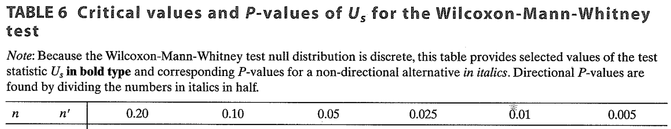
The critical value for would be greater than greater than 77, with an exact p-value of $p=.043$ for $U=77$. A formal statistical test in our software would reveal the same thing.

Rank Sum Test in R

In R, we can complete a Rank Sum Test using the stats package. Specifically, the function:

wilcox.test(DV ~ IV, data=your_data)

Where:

• DV is your DV, which can be ranked or unranked (R will rank for you)
• IV if your grouping variable
• your_data is replaced with your data.frame name

For us, the results would be:

    Wilcoxon rank sum exact test

data:  Rank by Group
W = 77, p-value = 0.04326
alternative hypothesis: true location shift is not equal to 0

22.3.1 Rank Sum Test - Write-up

Results

To examine the effect of competitive framing on cognitive performance, a Wilcoxon rank-sum test (Mann-Whitney U test) was conducted to compare task performance ranks between participants who received competitive instructions (control group) and those who received non-competitive instructions (experimental group). The results revealed a statistically significant difference in performance ranks between the two groups, $U=77$, $p=.043$. This suggests that the way the task was framed—as a race versus not a race—had a measurable impact on how participants performed. Specifically, participants in the non-competitive condition tended to perform worse than those in the competitive condition, despite completing the task in isolation. These findings support the hypothesis that competitive framing can influence cognitive task outcomes.

22.4 Wilcoxon’s Matched-Pairs Signed-Ranks Test

Sometimes we violate the assumptions of parametric tests like the paired t-test—such as the assumption of normality. In these cases, or when dealing with ordinal data, we can turn to nonparametric methods, like the Wilcoxon’s Matched-Pairs Signed-Ranks Test.

This test is used when each participant is measured twice (e.g., before and after a treatment), and we want to determine if there’s a statistically significant change in the direction and magnitude of their scores.

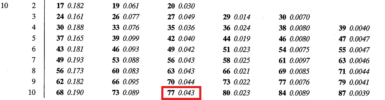
22.4.1 Paired Well-being: Pre- and post-COVID

Suppose we are studying how COVID-19 impacted high school students’ mental well-being. We assess the same group of students before the pandemic and again after restrictions were lifted. Mental well-being is measured using the Global Assessment of Functioning (GAF) scale, which was adjusted so that lower numbers reflect better functioning and higher numbers reflect worse functioning. We could only recruit 20 people, which was means our sample size is limiting and we have small statistical power (hypothetical power anlaysis suggests $n=112$). In this example:

• Independent Variable (IV): Time (Pre-COVID vs. Post-COVID)
• Dependent Variable (DV): Mental well-being (GAF scores)
• Design: Repeated measures (paired observations)

Here are the results:

After inspecting the data visually, we can tell the data are positively skewed and may not meet the assumptions of the paired samples t-test. A Shapiro-Wilks test revealed that our data are non-normally distributed (all $ps<.05$).

The signed rank test is similar to the rank sum test, with some minor adjustments. In short, the test is completed by:

1. Calculate difference scores for each participant.
2. Ignore zero differences.
3. Rank the absolute value of the differences.
4. Apply the sign of the original difference to the ranks.
5. Compute the sum of positive ranks and the sum of negative ranks.
6. The Wilcoxon test statistic, W (or V), is the smaller of these two sums.

• Note: some software will just use the value for the positive change ranks

We can summarize steps 1, 2, 3, and 4 in the following table:

We can then sum the ranks for the positive and negative ranks separately. Here, we get:

22.4.2 Critical Value

To determine significance, we can compare our observed $W$ (or $V$) to critical values in a Wilcoxon Signed-Ranks Table. For small samples (e.g., $n=15$), these tables provide exact values. Alternatively, software can compute exact p-values or use a normal approximation. Looking up our critical value here, we can see that for a sample size of 20, the $p<.05$ when $V<52$ (our smallest value is 16.5).

Signed Rank Test in R

You can perform the test in R using the same wilcox.test() function as above, but you need to specify that paired = TRUE. For example:

wilcox.test.(DV ~ IV, data = your_data, paired = TRUE, alternative = "two.sided")

For our data it would result in (and give an exact p-value):

    Wilcoxon signed rank test with continuity correction

data:  GAF by Time
V = 119.5, p-value = 0.007953
alternative hypothesis: true location shift is not equal to 0

22.4.3 When to Use

Use Wilcoxon’s Matched-Pairs Signed-Ranks Test when:

1. You have paired samples or repeated measures.
2. The assumption of normality is violated.
3. Your data are ordinal or you prefer a robust nonparametric method.

22.4.4 Signed Rank Test - Write-Up

Results

To examine the effect of time (pre- vs. post-COVID) on adolescent mental well-being, a Wilcoxon’s Matched-Pairs Signed-Ranks Test was conducted to compare Global Assessment of Functioning (GAF) scores before and after the onset of the COVID-19 pandemic. The results revealed a statistically significant difference in well-being scores across timepoints, $V=119.5$, $p=.008$. This suggests that students’ mental well-being changed significantly from pre- to post-COVID. Specifically, scores were higher after the onset of COVID-19, indicating an worsening in functioning. These findings suggest that some students may have experienced psychological impairments in the face of pandemic-related changes.

22.5 Kruskal-Wallis Test

There may be research scenarios where we have three or more groups and want to test differences on some ranked outcome. Here, the Kruskal-Wallis (KW) test is a suitable method to analyse the data. Conceptually, this test is similar to our previous non-parametric tests. Let’s work through an example.

22.5.1 Gatorade, Milk, or H20?

You are hired by the Canadian Olympic Committee to test the impacts of types of drinks prior to competition. They want to know if certain drinks increase performance during short races. You decide to help them by conducting a brief study. In this study, you aim to investigate whether the type of drink consumed prior to a 2km race impacts performance. You manage to recruit 15 lucky participants. Participants were randomly assigned to one of three conditions, which required them to drink 500mL of one of three liquids: Gatorade, milk, or water. After consuming their assigned beverage, all participants completed the race individually. Performance was measured by finishing place (i.e., rank), with lower ranks indicating faster times (i.e., first place ran the fastest). You hypothesize that individuals who drink Gatorade will perform better.

In this scenario, a KW test is suitable. It can be used to determine whether race ranks differed significantly across the three drink conditions (i.e., people who drink Gatorade typically rank higher).

In short, the Kruskal-Wallis test is a nonparametric alternative to one-way ANOVA, used when comparing three or more independent groups. The test is completed by:

1. Combine all scores from all groups into a single list.
   
2. Rank all values from lowest to highest, regardless of group.
   
3. Sum the ranks within each group.
   
4. Compute the Kruskal-Wallis H statistic, which evaluates how different the group rank sums are from what would be expected under the null hypothesis.
   
5. Compare the H statistic to a chi-square distribution with $k-1$ degrees of freedom (where $k$ is the number of groups).
   
6. If the result is statistically significant, it suggests that at least one group differs in median from the others.

After collecting data, we assign ranks (steps 1 and 2). We obtain the following data:

Here we have our ranks. For other contexts, you may need to manually assign ranks to the data.

For step 3, we will not calculate the sum of ranks for each group.

Next we calculate the $H$ statistic, which is defined as:

$$H=\frac{12}{N(N+1)}\sum _{i=1}^k\frac{T_i^2}{n_i}-3(N+1)$$

Where:

• $N$ is our total sample size;
• $n_i$ is the sample size for group $i$;
• $T_i$ is the sum of ranks for group $i$

So, for our data, the $H$ statistics can be calculated as:

$$\begin{gathered} H=\frac{12}{15(16+1)}\times (\frac{{33}^2}{5}+\frac{{63}^2}{5}+\frac{{24}^2}{5})-3(15+1) \\ =0.047\times (217.8+793.8+115.2)-48 \\ =56.34-48 \\ =8.34 \end{gathered}$$

Importantly, the $H$ statistics is distributed as a ${\chi }^2$ with $df=k-1$ ($k$ is the number of groups). Thus, we can compare to a critical ${\chi }^2$ value, as can be found on many websites), or calculate an exact p-value using statistical software. For example, in R:

pchisq(q = 8.34, df = 2, lower.tail = F)

Which results in:

[1] 0.01545226

KW Test in R

The KW test can be done using the rstatix package. The kruskal_test() function is similar to our Wilcox function:

kruskal_test(DV ~ Group, data=your_data)

The results from our example would be:

# A tibble: 1 × 6
  .y.       n statistic    df      p method        
* <chr> <int>     <dbl> <int>  <dbl> <chr>         
1 Place    15      8.34     2 0.0155 Kruskal-Wallis

22.5.2 KW Post-hoc Analyses

Like an ANOVA, the KW test is an omnibus test. It can tell us whether there is an overall difference between the groups, but does not let us know where it is. As a result, we need to conduct post-hoc analyses, which will compare the rankings of our various groups. This is primarily done through Dunn’s Test of Multiple Comparisons.

Dunn’s test provides a z-score for each group comparison. By now, you have a sound understanding of z-scores and their interpretations, including what may be considered an unlikely value. We can calculate Dunn’s test using the following:

$$z_i=\frac{y_i}{{\sigma }_i}$$ where:

• $z_i$ is the resulting z-score for comparison $i$
• $y_i$ is the difference in mean of the sum of the for two groups, ${\overline{W}}_A-{\overline{W}}_B$
• ${\sigma }_i$ is the standard error of the differences, which is given by:

$${\sigma }_i=\sqrt{\frac{N(N+1)}{12}-\frac{\sum _{s=1}^r{\tau }_s^3-{\tau }_s}{12(N-1)}(\frac{1}{n_i}+\frac{1}{n_j})\cdot C}$$

Wow. That’s a handful. Don’t worry, we will use our statistical software to calculate our resulting z-scores.

Dunn Test in R

The rstatix package also has a dunn_test() function. The structure is the same as we have encountered. I like to adjust using the Bonferroni correction. Also, setting detailed = T provides some other useful output.

dunn_test(DV ~ IV, data = your_data, p.adjust.method = 'bonferroni', detailed = T)

In the following, which is the results from our Gatorade, milk, and water example, ‘statistic’ is the z-score.

Here we want to focus on the adjusted p-value, which has the Bonferroni correction. As we can see, the only pairwise difference that is unlikely given the null is between the Milk and Water groups. Specifically, the water group finished faster than the milk group. The other comparisons were not unexpected under the null.

22.5.3 KW Test - Write-up

Results

The results of the Kruskal-Wallis test suggests that the ranks of the three groups unexpected given a true null hypothesis, ${\chi }^2(2)=8.34,p=.016,{\eta }_H^2=.528$.

Bonferroni-corrected post-hoc test were conducted to determine additional group differences. Specifically, post-hoc tests indicate that the milk group had lower rankings than the water group, $z=-2.76,p=.017$. However, the Gatorade group did not differ from the milk group, $z=-2.12,p=.102$, nor the water group, $z=-0.636,p>.999$.

22.6 Friedman Test

There may be research scenarios where we have three or more **repeated-measures* groups and want to test differences on some ranked outcome. Here, the Friedman test is a suitable method to analyse the data. Here, we have the same experimental units (e.g., people) measured multiple times with some ranked data.

22.6.1 Teaching Methods and Student Outcomes

You’re interested in evaluating how different teaching methods affect students’ performance. You recruit 10 undergraduate students, and each student receives instruction in three different teaching formats over the course of three weeks:

1. Traditional Lecture
2. Problem-Solving Workshop
3. Online Learning Module

After each session, students complete a standardized test designed to assess their understanding.

In short, the Friedman test is a nonparametric alternative to repeated-measures ANOVA, used when comparing three or more related (paired) groups. The test is completed by:

1. Organize the data so that each row represents a subject (or matched set), and each column represents a treatment or condition.
2. Rank the scores across each row (i.e., within each subject) from lowest to highest. Tied values receive average ranks.
3. Sum the ranks for each treatment condition (i.e., column-wise).
4. Compute the Friedman test statistic ($Q$ or ${\chi }_F^2$), which evaluates whether the rank sums differ more than expected by chance under the null hypothesis.
5. Compare the statistic to a chi-square distribution with ($k-1$) degrees of freedom (where $k$ is the number of conditions).
6. If the result is statistically significant, it suggests that at least one condition differs in its effect compared to the others.

We obtain the following data:

Unfortunately, due to our small sample size and non-normal data, we must rank the data. For step 1 and 2, we will rank each row’s (i.e., unit/person) data. Consider person 1–their highest score was problem based, followed by online, followed by lecture. Thus, they would receive rankings accordingly. Completing this for each row would result in (note that a rank of 1 indicates a ‘highest’ score).

Next we will sum the ranks of each treatment condition. Intuitively, this makes sense. If one method is superior, then the ranks should be higher (or lower, depending on how you coded) for that group. In our example, if Problem-Solving workshops are superior, people’s ranks should be more ‘1’ than ‘2’ or ‘3’. Thus, we we add the sum of ranks, if should be lower than the other groups.

When we add the sum of ranks for each group, we get:

The $Q$ (${\chi }_F^2$) statistic (with $df=k-1$) is defined as:

$${\chi }_F^2=\frac{12}{Nk(k+1)}\times (\sum R_i^2-3N(k+1))$$ Where:

• $R_i^2$ = squared sum of ranks for condition $i$
• $N$ is the number of participants
• $K$ is number of conditions/groups

For our example:

$${\chi }_F^2=\frac{12}{10(3)(4)}\times ({21}^2+{28}^2+{11}^2)-3(10)(4)$$

$$=0.1\times 1346-120$$

$$=14.6$$

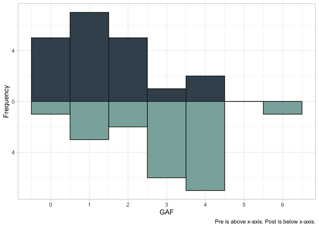
We can then compare this statistic to a critical value table or, more likely, get the exact p-value from our staitsitcal software. For example:

In the above image, we would look to $k$ (number of groups) and $n$ (total sample size). For us, the critical value at $\alpha =.05$ is ${\chi }_F^2=6.20$.

Friedman Test in R

It’s similar to our last tests–shocker! We would use the rstatix package and the friedman_test() function. The major difference is we need to specify our ID variable. We should have a column specifying the repeated treatment/group, a column for outcome, and a column for ID/participant specifier. Our function is specified as:

friedman_test(DV ~ IV | ID, data = your_data)

Alternatively, you could specify three columns, each representing the DV, IV, and ID for participants. For example:

friedman.test(your_data$DV, your_data$IV, your_data$ID)

Which, for our example, would result in:

# A tibble: 1 × 6
  .y.            n statistic    df        p method       
* <chr>      <int>     <dbl> <dbl>    <dbl> <chr>        
1 Test_Score    10      14.6     2 0.000676 Friedman test

22.6.2 Friedman Test - Effect Size

The typical effect size for the Friedman test is Kendall’s $W$, which is defined as:

$$W=\frac{{\chi }_f^2}{N(K-1)}$$

Kendall’s W has possible values of 0-1, with higher values indicating a higher effect size. For our data, the effect size is:

$$W=\frac{14.6}{10(3-1)}$$

$$W=.73$$ ### Friedman Post-hoc

Much like our KW test, we will need to conduct post-hoc comparisons to determine where the group differences lie. We can do this using Bonferroni-adjusted signed rank tests.

# A tibble: 3 × 9
  .y.        group1        group2    n1    n2 statistic     p p.adj p.adj.signif
* <chr>      <chr>         <chr>  <int> <int>     <dbl> <dbl> <dbl> <chr>       
1 Test_Score Lecture_Score Onlin…    10    10        52 0.014 0.043 *           
2 Test_Score Lecture_Score Probl…    10    10         1 0.004 0.012 *           
3 Test_Score Online_Score  Probl…    10    10         0 0.002 0.006 **          

22.6.3 Friedman - Write-up

We conducted a Friedman test to determine whether tests scores were associated with teaching method. The results suggest that test score ranking were statistically significantly associated with teaching method, ${\chi }_F^2=14.6,p<.001,W=.73$.

Post-hoc analysis were conducted using Bonferroni-adjusted signed rank tests. These results suggest that, first, students scored significantly higher following the problem-solving method compared to the lecture method, $V=1$, $p_{\text{adj}}=.012$. Second, the problem-solving method also significantly outperformed the online method, $V=0$, $p_{\text{adj}}=.006$. Last, scores following the lecture method were significantly higher than those following the online method, $V=52$,$p_{\text{adj}}=.043$.

Taken together, these results suggest that all three teaching methods yielded significantly different student outcomes, with the problem-solving approach consistently associated with better performance.

22.7 Practice

Practice Questions: Nonparametric Tests

1. A researcher wants to compare three independent groups using ordinal data. Which nonparametric test should they use?

2. You conduct a Friedman test on students’ scores across three different learning conditions and obtain a significant result. What post hoc test would be appropriate, and why?

3. What is the primary assumption difference between the Mann-Whitney U test and the Wilcoxon signed-rank test?

4. In the context of the Kruskal-Wallis test, why do we apply a tie correction to the standard error formula in post hoc tests?

5. Suppose you conduct multiple pairwise comparisons after a Friedman test. What correction method can you use to control for Type I error?

6. You find that the Wilcoxon signed-rank test statistic ( V ) = 0. What does this imply about your data?

7. Describe one situation where you would use the sign test instead of the Wilcoxon signed-rank test.

8. What are the null and alternative hypotheses for a Kruskal-Wallis test?

Answers

1. The Kruskal-Wallis test is appropriate for comparing three or more independent groups using ordinal data.

2. The Dunn-Bonferroni test is appropriate for pairwise comparisons following a significant Friedman test because it controls for Type I error in multiple comparisons using ranked data.

3. The Mann-Whitney U test compares independent samples, while the Wilcoxon signed-rank test is for paired or related samples.

4. A tie correction is applied because tied ranks reduce the variability in the rank distribution, which affects the accuracy of the standard error and p-value.

5. The Bonferroni correction (or Holm-Bonferroni) is commonly used to adjust p-values when conducting multiple pairwise comparisons.

6. A ( V ) value of 0 suggests that all participants scored higher (or lower) in one condition than the other, indicating a strong directional difference.

7. Use the sign test when the magnitude of differences isn’t meaningful or reliable, such as when data violate the assumptions of the Wilcoxon test (e.g., non-symmetric distributions).

8. Null hypothesis: All groups come from the same population (i.e., have the same median ranks).
   Alternative hypothesis: At least one group differs in its distribution (i.e., in median ranks) from the others.

22.8 Practice 2 - An Example

A health psychologist is studying whether different relaxation techniques affect self-reported anxiety levels. Each of 10 participants tries three different methods on separate days:

1. Deep breathing
   
2. Progressive muscle relaxation (PMR)
   
3. Mindfulness meditation

After each session, participants rate their anxiety level on a scale from 1 (no anxiety) to 10 (very anxious). The psychologist uses a Friedman test to determine whether there are statistically significant differences in anxiety ratings across the three techniques.

22.8.0.1 Participant Anxiety Ratings

Participant	Breathing	PMR	Mindfulness
1	5	4	3
2	6	5	4
3	7	6	4
4	4	3	2
5	5	4	2
6	6	5	3
7	7	6	5
8	6	5	3
9	5	4	3
10	4	3	2

Your Task

Use the data above to perform a Friedman test to determine whether anxiety levels differ across the three relaxation techniques.

• Step 1: Rank the anxiety ratings within each participant
  
• Step 2: Sum the ranks for each technique
  
• Step 3: Use the Friedman formula or statistical software to calculate the test statistic
  
• Step 4: Interpret the result

Answers

22.8.0.2 Step 1: Rank within each participant (lower anxiety = better)

Participant	Breathing	PMR	Mindfulness	R_Breathe	R_PMR	R_Mind
1	5	4	3	3	2	1
2	6	5	4	3	2	1
3	7	6	4	3	2	1
4	4	3	2	3	2	1
5	5	4	2	3	2	1
6	6	5	3	3	2	1
7	7	6	5	3	2	1
8	6	5	3	3	2	1
9	5	4	3	3	2	1
10	4	3	2	3	2	1

22.8.0.3 Step 2: Sum ranks for each condition

• Breathing: $3\times 10=30$
• PMR: $2\times 10=20$
• Mindfulness: $1\times 10=10$

22.8.0.4 Step 3: Friedman Test Formula

$${\chi }_F^2=\frac{12}{nk(k+1)}\sum R_j^2-3n(k+1)$$

$$=\frac{12}{10\cdot 3\cdot 4}({30}^2+{20}^2+{10}^2)-3\cdot 10\cdot 4$$

$$=\frac{12}{120}(900+400+100)-120=\frac{12}{120}(1400)-120=140-120=20$$

22.8.0.5 Step 4: Conclusion

With ${\chi }^2(2)=20.00$, $p<.001$, the Friedman test is significant. Anxiety levels significantly differed depending on the relaxation technique used. Post hoc comparisons would likely show that mindfulness resulted in lower anxiety ratings than either breathing or PMR.